Getting started with designbgm

library(designbgm)

designbgm plans the sample size of a prospective study for a Bayesian graphical model, given a prior elicited from a previous study. The inputs are a precision matrix K, its graph G, and the study size nu. If available, edge-inclusion probabilities pip can also be provided. The workflow is:

This vignette walks through this workflow on a real network, available from published data. The data are from Faelens, Hoorelbeke, Fried, De Raedt, & Koster (2019), “Negative influences of Facebook use through the lens of network analysis”, Computers in Human Behavior, 96, 13-22, openly available on OSF. The study has two samples: an exploratory one (N = 207) and a preregistered replication (N = 468). Each includes the following constructs:

FBI = Facebook use intensity
COMF = social comparison
RSES = global self-esteem
RRS = rumination
CSS = contingent self-esteem
MSFU_* = Facebook use style
Stress
Anxiety
Depression

First, we download the data locally from the OSF repository:

study1_csv <- tempfile(fileext = ".csv")
study2_csv <- tempfile(fileext = ".csv")
download.file("https://osf.io/download/hkctf/", study1_csv, mode = "wb", quiet = TRUE) # Data1_subscales.csv
download.file("https://osf.io/download/7fjge/", study2_csv, mode = "wb", quiet = TRUE) # Data2_subscales.csv
study1 <- read.csv2(study1_csv)
study2 <- read.csv2(study2_csv)
dim(study1)
#> [1] 207  11
dim(study2)
#> [1] 468  11

The plan is the following: Study 1 is our prior study. We elicit a prior distribution from it and quantify how much information it carries. We then plan the size of the prospective study (Study 2) using three planners, DPIR, BFDA, and BSDA. Finally, we compare the recommendations across all three planners to provide an illustrative walkthrough of Bayesian sample size determination.

Estimating a network (`ggm_parameters()`)

This section builds the inputs required by ggm_parameters(): a precision matrix K, a graph G, and inclusion probabilities pip. Because none of these are directly observed, they must first be estimated from Study 1’s data.

designbgm requires an already-estimated network rather than raw data. This estimate comes from a Bayesian fit: starting from a noninformative prior (a diffuse precision matrix and prior odds set to 0.5 for every edge), designbgm’s G-Wishart birth-death sampler updates based on Study 1’s data and returns a posterior precision matrix and posterior inclusion probabilities for every edge. We find the posterior structure graph G by thresholding each pip at 0.5 (the median probability model).

data1_norm <- suppressMessages(huge::huge.npn(study1)) # nonparanormal transform
#> Conducting the nonparanormal (npn) transformation via shrunkun ECDF....done.
X  <- scale(data1_norm)                                # center, unit variance
p  <- ncol(X)
n1 <- nrow(X)

nu0    <- p + 3L          # diffuse prior df, satisfying ggm_parameters()'s nu > p
scale0 <- diag(p)         # diffuse prior scale
D0     <- solve(scale0)
Dn     <- D0 + t(X) %*% X # posterior rate: prior + data's scatter matrix
plo0   <- matrix(0, p, p) # 0 = logit(0.5): uniform prior odds per edge

set.seed(202608)
fit1 <- designbgm:::cpp_bdmcmc_dcbf_sampler(
  n = n1, nu = nu0, D0 = D0, Dn = Dn, scale_prior = scale0, scale_post = solve(Dn),
  plo = plo0, G_start = matrix(0, p, p), n_iter = 100000L, n_burnin = 40000L,
  gwish_sampler = "direct", gwish_tol = 1e-8, gwish_iter = 500L, gwish_burnin = 500L)

nm <- names(study1)
G1 <- (fit1$pip > 0.5) * 1L # find posterior structure G by setting G_ij = 1 if PIP_ij > 0.5; 0 otherwise
diag(G1) <- 0
dimnames(G1) <- list(nm, nm)
K1 <- constrain_precision_to_graph(fit1$K_hat, G1) # clean numerical noise at non-edges
dimnames(K1) <- dimnames(G1)
pip1 <- fit1$pip
dimnames(pip1) <- dimnames(G1)
nu1  <- nu0 + n1 # posterior df (degrees of freedom): this posterior is the prior for planning Study 2

sum(G1) / 2 # edges
#> [1] 18

K1 and G1 are what ggm_parameters() needs below, and nu1 is the study size (a posterior built from a noninformative prior plus n1 observations for planning purposes behaves like an elicited prior of size nu0 + n1). Below, the plot of the network directly from K1, where: edge width scales with |partial correlation|, edge color encodes its sign, and node placement comes from a layout that pulls strongly-connected nodes together.

Rho1 <- designbgm:::cpp_precision_to_partial_correlations(K1)
dimnames(Rho1) <- dimnames(K1)

g1 <- igraph::graph_from_adjacency_matrix(G1, mode = "undirected", diag = FALSE)
el <- igraph::as_edgelist(g1, names = TRUE)
edge_rho <- Rho1[cbind(el[, 1], el[, 2])]
igraph::E(g1)$weight <- edge_rho
igraph::E(g1)$width  <- 1 + 6 * abs(edge_rho) / max(abs(edge_rho))
igraph::E(g1)$color  <- ifelse(edge_rho > 0, "#3182bd", "#de2d26")

igraph::V(g1)$size        <- 20
igraph::V(g1)$color       <- "#abd9e9"
igraph::V(g1)$label.cex   <- 0.75
igraph::V(g1)$label.color <- "black"
igraph::V(g1)$frame.color <- "white"

set.seed(18)
lay <- igraph::layout_with_fr(g1, weights = 1 + 5 * abs(igraph::E(g1)$weight), niter = 5000)

par(mar = c(3, 1, 1, 1))
plot(g1, layout = lay, edge.curved = 0.15, xlim = c(-1.3, 1.3), ylim = c(-1.3, 1.3))
legend("bottom", inset = c(0, -0.12), bty = "n", cex = 0.7, lwd = 3, horiz = TRUE, xpd = TRUE,
       col = c("#3182bd", "#de2d26"), legend = c("positive edge", "negative edge"))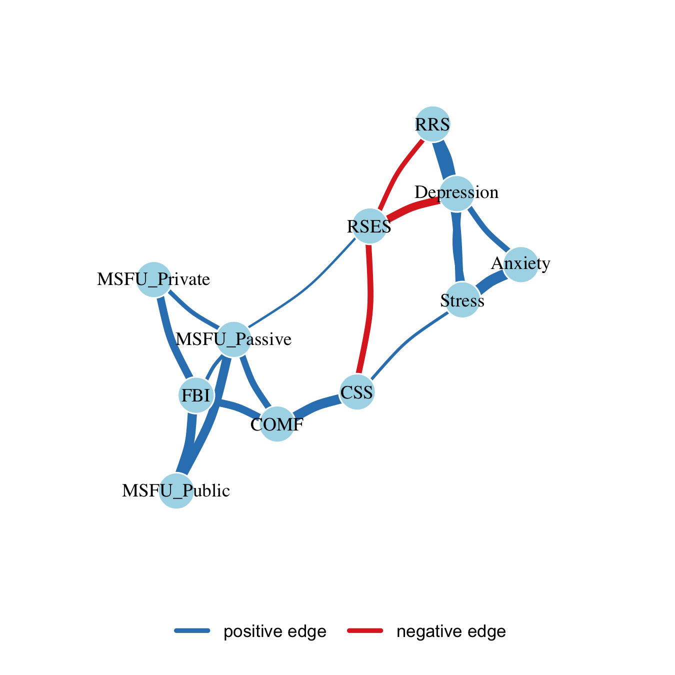

Sorting the present edges by |partial correlation| will be useful later:

Gu  <- G1; Gu[lower.tri(Gu)] <- 0
idx <- which(Gu == 1, arr.ind = TRUE)
edge_tab <- data.frame(
  var1 = rownames(K1)[idx[, 1]], var2 = colnames(K1)[idx[, 2]],
  i = idx[, 1], j = idx[, 2], rho = Rho1[idx]
)
edge_tab$abs_rho <- abs(edge_tab$rho)
edge_tab <- edge_tab[order(edge_tab$abs_rho), ]
nrow(edge_tab)
#> [1] 18

Eliciting the prior (`elicit_prior()` and `prior_ess()`)

params1   <- ggm_parameters(K = K1, G = G1, nu = nu1, pip = pip1)
elicited1 <- elicit_prior(params1)
elicited1
#> <ggm_elicited>  prior: gwishart 
#>   nodes : 11 
#>   edges : 18 of 55 
#>   nu    : 221  (prior study size)
#>   pip   : matrix, range [0.034, 1.000]

How much information does this prior carry?

pe <- prior_ess(elicited1)
pe
#> <prior_ess>  family: ggm  prior: gwishart 
#>   VR    : 322.833
#>   PR    : 202.932
#>   MTM   : 220
#>   PT    : 209
#>   ELIR  : 209

ess_vals <- vapply(pe$estimates, function(x) x$global, numeric(1))
barplot(ess_vals, col = "steelblue", ylab = "prior ESS",
        main = "Prior effective sample size, by estimator")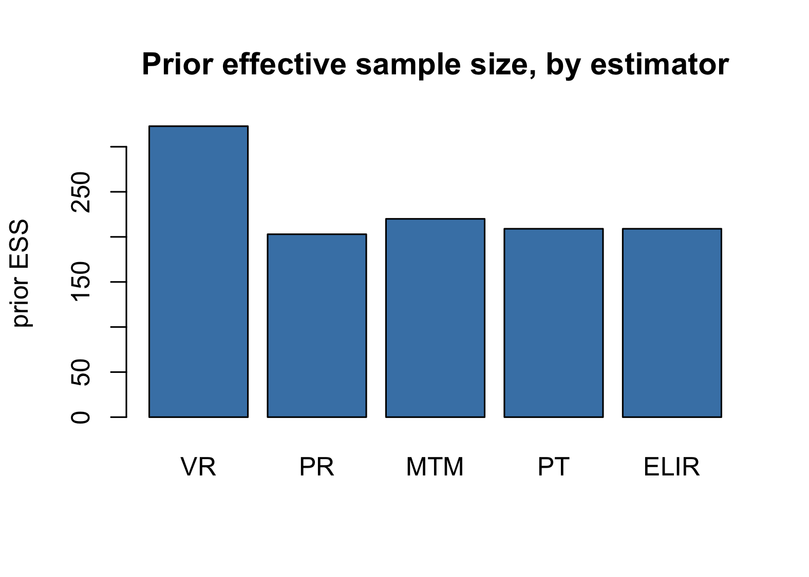

Prior ESS measures how much information the elicited prior carries, in observation-equivalent units: it does not necessarily equal nu1, the prior’s degrees of freedom, because the entries of the precision matrix are coupled through complex dependencies. Two of the estimators above bound the prior study size on either side, PR < nu1 < VR, and PR tends to be more stable and less sensitive to prior instability than VR (where by instability we refer to that in the prior’s covariance or Fisher information matrix, to which VR is more exposed).

Prior uncertainty (visualized)

Prior ESS is a lower bound on how big the next study should be, but it collapses a much richer object into one number: the elicited prior is not a single value for each partial correlation, it is a distribution with actual spread around it. While the ESS summary quantifies the information contained in the prior study, design() accounts for the prior uncertainty when it plans. Below, the posterior distribution of the network’s strongest edge, drawing directly from the elicited G-Wishart prior:

strongest <- edge_tab[nrow(edge_tab), ]
strongest[, c("var1", "var2", "rho")]
#>      var1    var2       rho
#> 14 Stress Anxiety 0.4609911

draws <- designbgm:::cpp_rgwishart(
  n = 5000L, K = elicited1$scale, nu = elicited1$nu, G = elicited1$G,
  sampler = "direct", tol = 1e-8, itermax = 500L, burnin = 500L, init = NULL)

i <- strongest$i; j <- strongest$j
prior_rho <- -draws[i, j, ] / sqrt(draws[i, i, ] * draws[j, j, ])
sd(prior_rho)
#> [1] 0.05024941

plot(density(prior_rho), main = sprintf("Prior belief: %s-%s", strongest$var1, strongest$var2),
     xlab = "partial correlation",lwd=2)
abline(v = strongest$rho, lty = 2)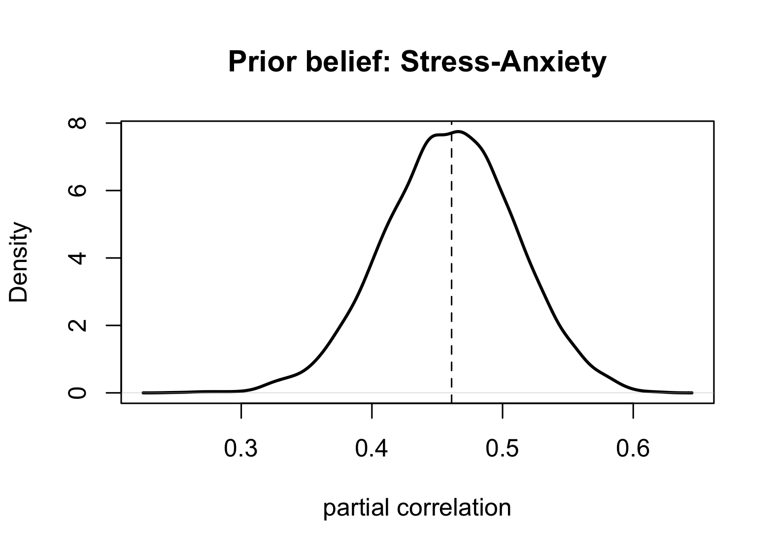

The prior is centered close to the point estimate from K1 (the dashed line), with a spread that design() and power_curve() account for when they simulate from it.

Planning a sample size (`design()`)

design() offers three planners for a Gaussian graphical model:

DPIR (Data-to-Prior Information Ratio) targets the precision matrix as a whole, asking how much data is needed for the data’s information to reliably outweigh the prior’s, both overall and for the off-diagonal parameters.
BFDA (Bayes Factor Design Analysis) targets a single representative edge, asking how much data is needed to reliably detect or exclude it via a Bayes factor.
BSDA (Bayesian Structural Design Analysis) targets the whole graph at once, asking how much data is needed to reliably recover edges at a target sensitivity or specificity.

The three sections below walk through each planner in turn.

Planning a sample size: DPIR

DPIR compares the data’s information about the precision matrix to the prior’s information, parameter by parameter, and asks how much data is needed for that ratio to reliably exceed a threshold (threshold = 1, data at least as informative as the prior, by default). It reports two sizes: global, for the precision matrix as a whole, and parameterwise, for whichever off-diagonal entry needs the most data to reach the threshold.

plan_dpir <- design(elicited1, method = "DPIR", H = 50, J = 10, max_n = 1500, n_tol = 5)
plan_dpir
#> <design>  method: DPIR  family: ggm  prior: gwishart 
#>   planned sample size (DPIR determinant ratio):
#>     global : n* = 236   (Pr(DPIR > threshold) = 0.960)
#>     weakest parameter : n* = 272

Because it targets every parameter rather than one representative edge or the graph’s structure, DPIR’s recommendation reflects the full precision matrix, rather than being restricted to single edges like in BFDA. Calling power_curve() plots two curves against n: the same global probability design() searches over, and the average probability across off-diagonal parameters.

n_grid_dpir <- c(50, 100, 130, 160, 190, 220, 250, 300, 400)
curve_dpir  <- power_curve(elicited1, method = "DPIR", n = n_grid_dpir, H = 50, J = 10)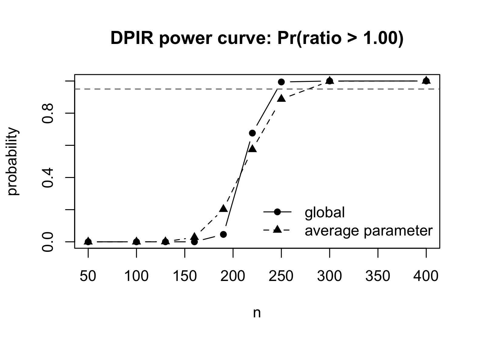

plot(curve_dpir)
abline(h = 0.95, lty = 2, col = "gray40")

Planning a sample size: BFDA

BFDA plans around a single representative edge, searching for the smallest sample size at which a Bayes factor reliably detects it (H1) or excludes it (H0), each at a target power. Because sample size requirements depend heavily on effect size, researchers typically select edge values or partial correlation thresholds that are motivated by theory or prior literature. To help guide this selection, the summary below provides sample size estimates across the 25th, 50th, and 75th percentiles of |partial correlation| among the present edges.

q     <- quantile(edge_tab$abs_rho, probs = c(0.25, 0.5, 0.75))
pick  <- vapply(q, function(target) which.min(abs(edge_tab$abs_rho - target)), integer(1))
target_edges <- edge_tab[pick, ]
target_edges
#>            var1        var2 i  j        rho   abs_rho
#> 2          RSES         RRS 3  4 -0.1589911 0.1589911
#> 17       Stress  Depression 9 11  0.2668532 0.2668532
#> 11 MSFU_Passive MSFU_Public 6  8  0.3678839 0.3678839

By default, design() picks an edge automatically via rho_quantile (the median edge, rho_quantile = 0.5):

design(elicited1, method = "BFDA", H = 50, J = 10, max_n = 1500, n_tol = 5)
#> <design>  method: BFDA  family: ggm  prior: gwishart 
#>   planning edge: (1, 2)   rho = 0.296
#>   planned sample size (Bayes factor):
#>     H0 (edge absent)  : n* = 79   (power = 0.818)
#>     H1 (edge present) : n* = 72   (power = 0.820)

To plan around a specific edge instead, pass edge (1-based node indices) directly, bypassing rho_quantile. Furthermore, one can set threshold, pow0, or pow1 explicitly or leave them at their default values: a Bayes factor of 10 (decisive evidence, in either direction) at 80% power (pow0 = pow1 = 0.8).

plans <- lapply(seq_len(nrow(target_edges)), function(k)
  design(elicited1, method = "BFDA", edge = c(target_edges$i[k], target_edges$j[k]),
         H = 50, J = 10, max_n = 1500, n_tol = 5))

bfda_summary <- data.frame(
  edge    = paste(target_edges$var1, target_edges$var2, sep = "-"),
  abs_rho = round(target_edges$abs_rho, 3),
  n_star_h0 = vapply(plans, function(p) if (isTRUE(p$results$converged_h0)) p$results$n_star_power_h0 else NA_real_, numeric(1)),
  n_star_h1 = vapply(plans, function(p) if (isTRUE(p$results$converged_h1)) p$results$n_star_power_h1 else NA_real_, numeric(1))
)
bfda_summary
#>                       edge abs_rho n_star_h0 n_star_h1
#> 1                 RSES-RRS   0.159       960       661
#> 2        Stress-Depression   0.267       284        22
#> 3 MSFU_Passive-MSFU_Public   0.368        89        42

A search that fails to converge within the cap (max_n = 1500) is itself informative as it indicates that the target edge requires a larger sample size than evaluated.

Power curves (`power_curve()`)

design() searches for the smallest n that reaches a target power. power_curve() instead evaluates the power at a grid of sample sizes. For a single edge, a grid tailored to where its curve actually moves is more informative than a generic one:

n_grid_single <- c(50, 150, 300, 450, 600, 750, 900, 1100, 1400, 1800)
curve_single  <- power_curve(elicited1, method = "BFDA", n = n_grid_single,
                             edge = c(target_edges$i[1], target_edges$j[1]), H = 50, J = 10)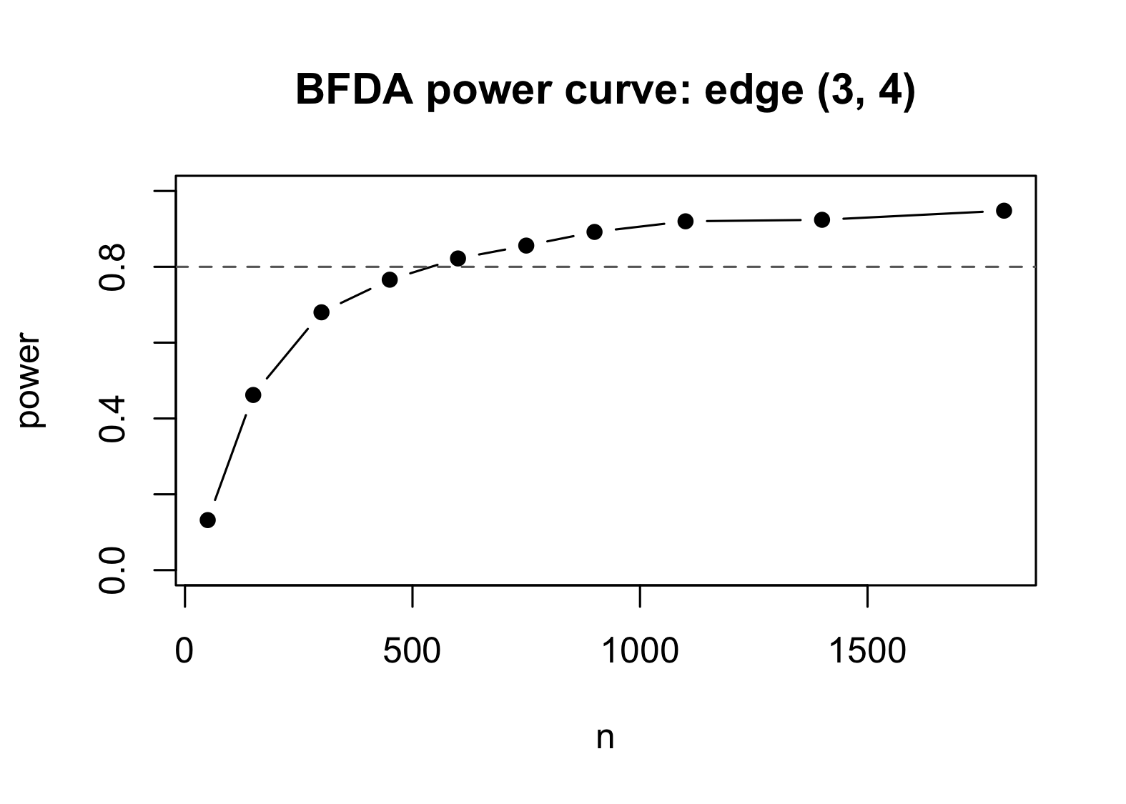

plot(curve_single)
abline(h=0.8,lty=2,col="gray40")

power_curve() returns a plain table, so comparing edges on one plot is straightforward. Here the three edges span a wider range of n*, so we define a wider grid:

n_grid <- c(20, 40, 80, 150, 250, 400, 650, 1000, 1500)

curves <- lapply(seq_len(nrow(target_edges)), function(k)
  power_curve(elicited1, method = "BFDA", n = n_grid,
              edge = c(target_edges$i[k], target_edges$j[k]), H = 50, J = 10))

cols <- c("#1b9e77", "#d95f02", "#7570b3")
plot(n_grid, curves[[1]]$results$table$power_h1, type = "b", pch = 16, col = cols[1],
     ylim = c(0, 1), xlab = "n", ylab = "power (H1: edge present)",
     main = "BFDA power to detect each edge")
lines(n_grid, curves[[2]]$results$table$power_h1, type = "b", pch = 16, col = cols[2])
lines(n_grid, curves[[3]]$results$table$power_h1, type = "b", pch = 16, col = cols[3])
abline(h = 0.8, lty = 3, col = "gray70")
legend("bottomright", bty = "n", cex = 0.8, col = cols, pch = 16, lty = 1,
       legend = paste0(target_edges$var1, "-", target_edges$var2,
                        "  (|rho|=", round(target_edges$abs_rho, 3), ")"))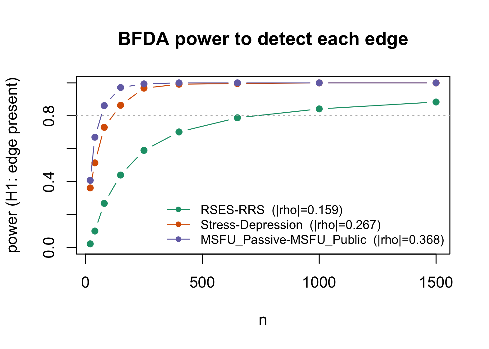

Planning a sample size: BSDA

BFDA plans around one edge. design(method = "BSDA") targets a different, stricter criterion: a sensitivity or specificity value (edge selection accuracy across the whole graph, not one edge), reached with a given power. It needs pip, already part of elicited1, and only applies to sparse graphs.

While all the planners sample parameters from the elicited prior to generate datasets, BSDA additionally fits a full posterior model (a birth-death MCMC run), estimating the posterior graph structure at every iteration. In the code below, bsda_control() specifies 4,000 iterations following a 2,000-iteration burn-in, while design() uses H = 150 prior draws.

bsda_ctrl <- bsda_control(H_scout = 30, n_scout = 5, n_main = 5,
                          fit_iterations = 4000, fit_burnin = 2000,
                          gwish_iter = 100, gwish_tol = 1e-2,
                          n_boot = 1000, max_iter = 4, verbose = FALSE, init = "empty")

set.seed(202608)
plan_bsda <- design(elicited1, method = "BSDA",
                    measure = "sen", measure_value = 0.8, target_pow = 0.8,
                    max_n = 8000, H = 150, J = 1, control = bsda_ctrl, range_lower = 200)
plan_bsda
#> <design>  method: BSDA  family: ggm  prior: gwishart 
#>   criterion: sen = 0.800, target power = 0.800
#>   planned sample size: n* = 5882   CI[4219, 10696]

The recommended sample size is far larger than the BFDA targets for the three edges above. This is expected: recovering the whole network reliably is a harder task than detecting one representative edge, provided that MCMC convergence (here using short chains of 6,000 total iterations) is verified across network sizes. However, this pattern does not hold for every edge. The weakest edges in the graph (not shown above) may require just as much data as BSDA, since the cost of BFDA grows as the effect size shrinks.

As with BFDA, power_curve() evaluates the power at a grid of sample sizes instead of searching for n*. Sensitivity and specificity each requires a separate function call:

n_grid_bsda <- c(500, 1000, 2000, 3500, 5500, 8000)

set.seed(202608)
curve_sen <- power_curve(elicited1, method = "BSDA", n = n_grid_bsda, H = 150, J = 1,
                         measure = "sen", measure_value = 0.8, control = bsda_ctrl)
set.seed(202608)
curve_spe <- power_curve(elicited1, method = "BSDA", n = n_grid_bsda, H = 150, J = 1,
                         measure = "spe", measure_value = 0.8, control = bsda_ctrl)

In power_curve(), the power column represents the probability of surpassing a threshold (Pr(measure >= measure_value)):

plot(n_grid_bsda, curve_sen$results$table$power, type = "b", pch = 16, col = "firebrick",
     ylim = c(0, 1), xlab = "n", ylab = "achieved value", main = "BSDA: Pr(measure >= 0.8)")
lines(n_grid_bsda, curve_spe$results$table$power, type = "b", pch = 17, col = "darkblue")
abline(v = plan_bsda$results$n_star, lty = 2, col = "gray40")
legend("right", bty = "n", pch = c(16, 17), col = c("firebrick", "darkblue"),
       legend = c("sensitivity", "specificity"))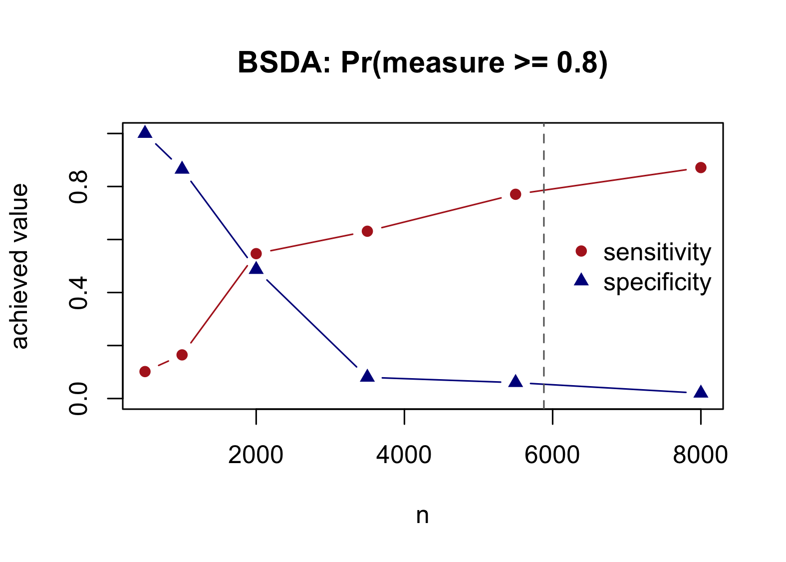

Paralell to this figure, one can also plot the measure_achieved column, which is the average measure value observed over a grid of sample sizes:

plot(n_grid_bsda, curve_sen$results$table$measure_achieved, type = "b", pch = 16, col = "firebrick",
     ylim = c(0, 1), xlab = "n", ylab = "achieved value", main = "BSDA: achieved sensitivity and specificity")
lines(n_grid_bsda, curve_spe$results$table$measure_achieved, type = "b", pch = 17, col = "darkblue")
abline(v = plan_bsda$results$n_star, lty = 2, col = "gray40")
legend("right", bty = "n", pch = c(16, 17), col = c("firebrick", "darkblue"),
       legend = c("sensitivity", "specificity"))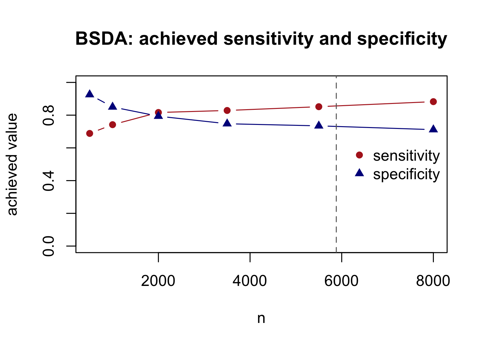

Sensitivity rises with n, as expected. Specificity moves the other way, falling as n grows: as more data comes in, it outweighs the prior more and more, and for this network that means the model starts including extra edges beyond the ones in G1. This sensitivity/specificity trade-off is a real, known property of network edge-selection methods.

Validating a plan (`validate()`)

Both design() and power_curve() estimate power using the same replicates drawn during the sample size search or grid evaluation. validate() closes the loop by re-evaluating the plan’s claimed power (or achieved measure) at its n* using an independent set of replicates.

Validating a plan: DPIR

which_n defaults to "global" for a DPIR plan; pass which_n = "pw" to validate the stricter, weakest-parameter size instead.

validate(plan_dpir, H = 100, J = 20)
#> <design_validation>  method: DPIR   n* = 236 
#>   global Pr(DPIR > threshold) at n* : 0.951
#>   parameterwise Pr at n* : min 0.669 / median 0.761 / max 0.797

Validating a plan: BFDA

validate(plans[[2]], H = 100, J = 20)
#> <design_validation>  method: BFDA   n* = 22 
#>   planning edge (9, 11): power_h0 = 0.573  power_h1 = 0.320

Validating a plan: BSDA

set.seed(202608)
validate(plan_bsda, H = 300, J = 1)
#> <design_validation>  method: BSDA   n* = 5882 
#>   criterion: sen = 0.800, target power = 0.800
#>   achieved power at n* = 5882 : 0.825 +/- 0.057
#>   target not met at n*

validate()’s “target met” check is conservative: it asks whether the lower end of the estimated power’s interval surpasses the target, not just whether the target falls inside the interval.

Summary: Synthesizing Planner Decisions with Prior ESS

The three planners evaluate prospective sample size requirements under distinct statistical targets, while all propagating the same information carried by the elicited prior. In the example above, DPIR requires a modest sample size to ensure that new empirical data outweighs the information carried by the elicited prior. In contrast, BFDA targets specific edges with sample size requirements that scale inversely with effect size, while BSDA demands a substantially larger sample to reliably recover overall graph topology (with performance depending on the convergence of the birth-death sampler).

Beyond the example presented in this vignette, researchers should select one or more planners based on their specific research goals: whether they seek only to outweigh prior information (DPIR) or also wish to guarantee evidence-based conclusions (BFDA or BSDA).

Furthermore, we stress that the estimated sample size in the presence of informative priors depends directly on the size of the prior study itself. A large prior study may allow for smaller prospective sample sizes under BFDA planners, yet at that smaller size, DPIR may not reach its target threshold, allowing prior information to dominate the posterior. Therefore, to ensure both prior dominance and decisive evidence, we recommend combining BFDA or BSDA with DPIR analysis and planning for the most conservative n*, provided it remains within the practical time and cost constraints of the study.

References

Arena, G., et al. (2026). What is your Prior Worth? Effective Sample Size and Sample Size Planning for Gaussian Graphical Models. arXiv. arXiv:2606.22687
Faelens, L., Hoorelbeke, K., Fried, E. I., De Raedt, R., & Koster, E. H. W. (2019). Negative influences of Facebook use through the lens of network analysis. Computers in Human Behavior, 96, 13-22. https://doi.org/10.1016/j.chb.2019.02.002 Data: https://osf.io/v7gch/

Estimating a network (ggm_parameters())

Eliciting the prior (elicit_prior() and prior_ess())