Power curve for a Gaussian graphical model (DPIR, BFDA, or BSDA)
Source:R/family-ggm.R
power_curve.ggm_elicited.RdEvaluates power at a grid of sample sizes without searching
for n*. Use together with plot() to see how power changes
with n. "DPIR" evaluates Pr(DPIR > threshold) both
globally and averaged across off-diagonal parameters (unlike
design's "pw" target, which is the weakest
off-diagonal parameter, not the average); "BFDA" evaluates power
and error rate for a single edge; "BSDA" evaluates
Pr(measure >= measure_value) over the whole graph.
Usage
# S3 method for class 'ggm_elicited'
power_curve(
  params,
  method = c("DPIR", "BFDA", "BSDA"),
  n,
  target_probability = 0.95,
  edge = NULL,
  rho_quantile = 0.5,
  pow0 = 0.8,
  pow1 = 0.8,
  threshold = NULL,
  measure = c("sen", "spe"),
  measure_value = 0.8,
  control = bsda_control(),
  H = 150L,
  J = 20L,
  ...
)
Arguments
- params
A
ggm_elicitedobject, as returned byelicit_prior. It also inherits frombgm_elicited.- method
Which planning method,
"DPIR"(default),"BFDA", or"BSDA".- n
Candidate sample sizes to evaluate (numeric vector).
- target_probability
DPIR only, as in
design. Not used in the grid computation itself (there is no search to stop); kept for the target reference line inplot()andprint().- edge
BFDA only: a length-2 integer vector, 1-based indices into the rows/columns of
KandGas supplied toggm_parameters, naming the edge to evaluate. The edge must be present inG. Order does not matter: the pair is sorted internally, since the underlying Bayes factor computation requiresm < l.NULL(default) selects viarho_quantile, as indesign.- rho_quantile, pow0, pow1
BFDA only, as in
design.- threshold
DPIR and BFDA only, as in
design.NULL(default) uses 1.0 for DPIR and 10.0 for BFDA.- measure, measure_value
BSDA only: the measure to evaluate (
"sen"or"spe") and the target value of that measure, as indesign.senandspeare evaluated by separate calls (they are two different computations, not two outputs of the same one); callpower_curve()twice to get both.- control
BSDA only: a list of control parameters, as returned by
bsda_control. Defaultbsda_control().- H, J
Outer and inner Monte Carlo replication counts, as in
design.- ...
Ignored, present for consistency with the generic
power_curve().
Value
A ggm_power_curve object, which also inherits from
bgm_power_curve. Its results$table component is a
data.frame with one row per n: for DPIR, n,
prob_global, prob_pw_mean (the average, across
off-diagonal parameters); for BFDA, n, power_h0, fpr_h0,
power_h1, fnr_h1; for BSDA, n, power,
measure_achieved, halfwidth, se. print and
plot methods are available.
See also
Other sample size planning:
bsda_control(),
design(),
design.ggm_elicited(),
power_curve(),
validate(),
validate.ggm_design()
Examples
p <- 3
G <- matrix(0, p, p)
G[1, 2] <- G[2, 1] <- 1
K <- diag(p)
K[1, 2] <- K[2, 1] <- 0.3
ep <- elicit_prior(ggm_parameters(K, G, nu = 10))
# DPIR (the default method)
set.seed(12)
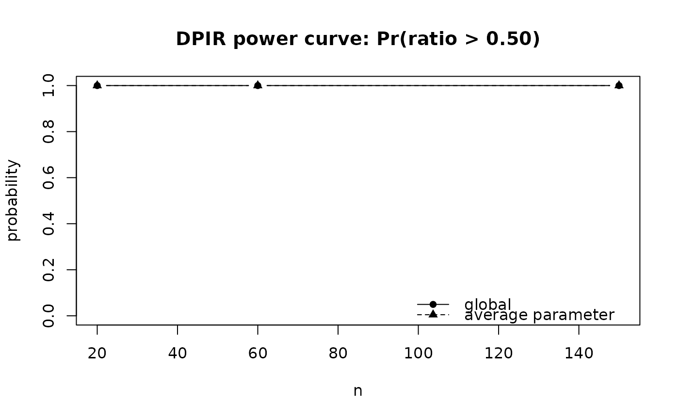
pc <- power_curve(ep, method = "DPIR", n = c(20, 60, 150), threshold = 0.5, H = 30, J = 10)
pc
#> <power_curve> method: DPIR family: ggm prior: gwishart
#> criterion: DPIR > 0.500 (target probability = 0.95)
#> n prob_global prob_pw_mean
#> 20 1 1
#> 60 1 1
#> 150 1 1
plot(pc)
 # \donttest{
# BFDA: plans around a single edge
set.seed(12)
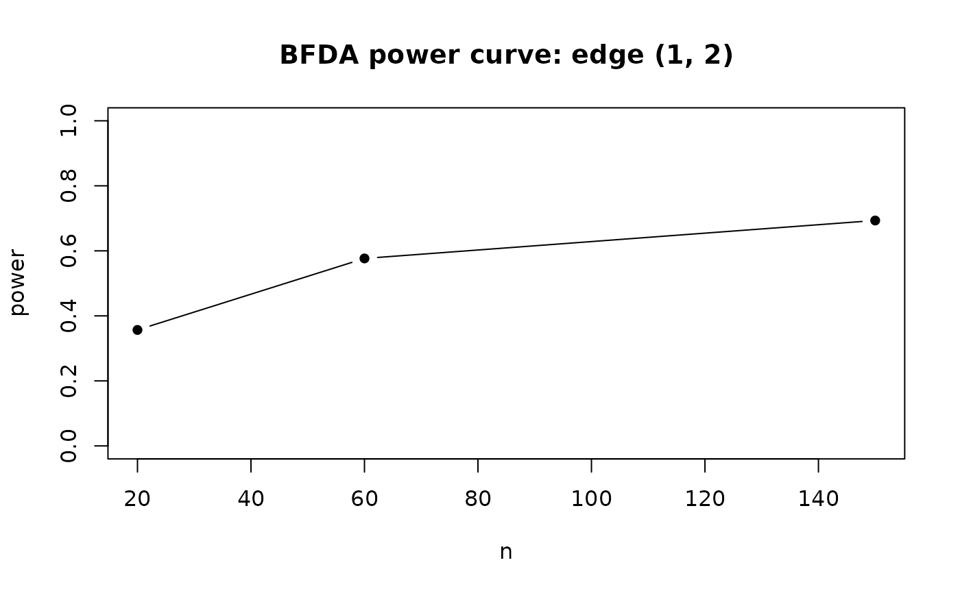
pc_bfda <- power_curve(ep, method = "BFDA", edge = c(1, 2), n = c(20, 60, 150), H = 30, J = 10)
plot(pc_bfda)
# \donttest{
# BFDA: plans around a single edge
set.seed(12)
pc_bfda <- power_curve(ep, method = "BFDA", edge = c(1, 2), n = c(20, 60, 150), H = 30, J = 10)
plot(pc_bfda)
 # BSDA: needs pip and a sparse graph. Here, control() settings are kept light
ep_pip <- elicit_prior(ggm_parameters(K, G, nu = 10, pip = 0.5))
ctrl <- bsda_control(
fit_iterations = 300, fit_burnin = 150, n_boot = 200,
gwish_iter = 80
)
set.seed(12)
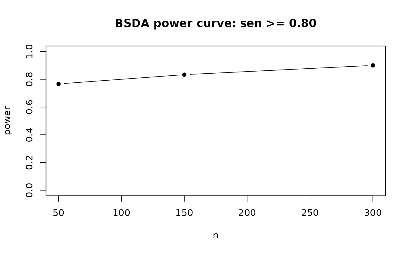
pc_bsda <- power_curve(ep_pip,
method = "BSDA", n = c(50, 150, 300), H = 30, J = 1,
measure = "sen", measure_value = 0.8, control = ctrl
)
plot(pc_bsda)
# BSDA: needs pip and a sparse graph. Here, control() settings are kept light
ep_pip <- elicit_prior(ggm_parameters(K, G, nu = 10, pip = 0.5))
ctrl <- bsda_control(
fit_iterations = 300, fit_burnin = 150, n_boot = 200,
gwish_iter = 80
)
set.seed(12)
pc_bsda <- power_curve(ep_pip,
method = "BSDA", n = c(50, 150, 300), H = 30, J = 1,
measure = "sen", measure_value = 0.8, control = ctrl
)
plot(pc_bsda)
 # }
# }