MCMC Diagnostics

Before interpreting results from bgm() or bgmCompare(), check that the MCMC sampler has converged and that posterior estimates are reliable. This chapter describes how to do so with the diagnostic tools in bgms. For background on MCMC convergence diagnostics and choosing the number of iterations, chains, and warmup length, see Margossian & Gelman (2024).

Effective sample size (ESS)

The effective sample size estimates how many independent draws the MCMC chain is equivalent to. Correlated draws reduce the effective information per sample. A larger ESS means more precise posterior estimates (Margossian & Gelman, 2024).

The summary() output reports n_eff for each parameter. How large n_eff needs to be depends on the inferential goal. As a rule of thumb, an ESS of 100 yields an MCSE of roughly $0.1$ times the posterior standard deviation — enough for one significant digit of precision. An ESS below 100 is also the threshold at which convergence diagnostics such as $\hat{R}$ and the ESS estimate itself become unreliable (Margossian & Gelman, 2024; Vehtari et al., 2021). If higher precision is required, more iterations or chains are needed: two significant digits require an ESS on the order of 10,000 (Margossian & Gelman, 2024).

Mixture ESS for edge-selected parameters

When edge selection is active, pairwise effects are governed by spike-and-slab priors. The parameter is set to exactly zero when the edge is excluded, creating a chain that mixes between zero and nonzero values.

Two ESS measures are reported:

n_eff: the unconditional ESS, computed from the full chain (including zeros). Measures how precisely the overall posterior mean is estimated.
n_eff_mixt: the mixture ESS, which accounts for additional uncertainty from the spike-and-slab switching. Suppressed in printed output when the total number of indicator transitions ($n_{0 \to 1} + n_{1 \to 0}$) is below 5, though still computed and stored.

The mixture ESS is derived from a two-state Markov chain representation of the indicator sequence (van den Bergh et al., 2026). Let $a$ denote the probability of switching from excluded to included ($0 \to 1$) and $b$ the probability of switching from included to excluded ($1 \to 0$). The lag-$k$ autocorrelation of the indicator chain is $\rho(k) = (1 - a - b)^k$, which gives an integrated autocorrelation time of $\tau = (2 - a - b) / (a + b)$ and an effective sample size of $\text{ESS} = T \cdot (a + b) / (2 - a - b)$. In practice, $a$ and $b$ are estimated from the observed transition counts $n_{01}$, $n_{00}$, $n_{10}$, and $n_{11}$.

Limitations near the boundary

The two-state Markov chain ESS has known limitations when the inclusion probability is near 0 or 1. In these cases the indicator is almost always in the same state, so transitions are rare and the estimates $\hat{a}$ and $\hat{b}$ are based on very few events. A single extra transition can change the ESS estimate substantially, making it unreliable as a precision diagnostic. For this reason, n_eff_mixt is suppressed in printed output when the total number of transitions is below 5.

At the extreme — when the indicator never switches — there are no transitions to estimate from. This does not necessarily indicate a problem: if the posterior strongly favors inclusion or exclusion, there is little uncertainty about the indicator and the inclusion probability is well determined even without switching.

When transitions are observed but rare, the ESS estimate itself becomes imprecise. The transition probability estimates $\hat{a}$ and $\hat{b}$ are each based on only a few events, giving them high relative error. Because the ESS formula $T (a + b) / (2 - a - b)$ depends on their sum, small fluctuations in the transition counts can produce large swings in the ESS. In these cases, plotting the cumulative inclusion probability across iterations provides a more informative check on stability: a flat trajectory indicates the estimate has settled, while a drifting one suggests the chain needs more iterations.

Monte Carlo standard error (MCSE)

The MCSE measures the additional variability introduced by using a finite number of MCMC draws instead of the exact posterior. It depends on both the posterior variability and the effective sample size.

For continuous parameters: \[ \text{MCSE} = \frac{\text{sd}}{\sqrt{n_{\text{eff}}}} \]

For inclusion probabilities, the posterior variance has the Bernoulli form $\hat{p}(1 - \hat{p})$, so: \[ \text{MCSE}(\hat{p}) = \sqrt{\frac{\hat{p}(1 - \hat{p})}{\text{ESS}}} \]

A small MCSE relative to the posterior standard deviation indicates stable estimates; a large MCSE suggests that more iterations are needed.

R-hat

R-hat (split R-hat) compares the between-chain and within-chain variance (Gelman & Rubin, 1992). Values close to 1.0 indicate that the chains have converged to the same distribution. Earlier guidance recommended thresholds of 1.1 or 1.2; Vehtari et al. (2021) tightened this to 1.01 based on experience with rank-normalized split-R-hat. Values above 1.01 suggest that the chains have not mixed and should be run longer.

bgms reports R-hat in summary() output and through extract_rhat().

Trace plots

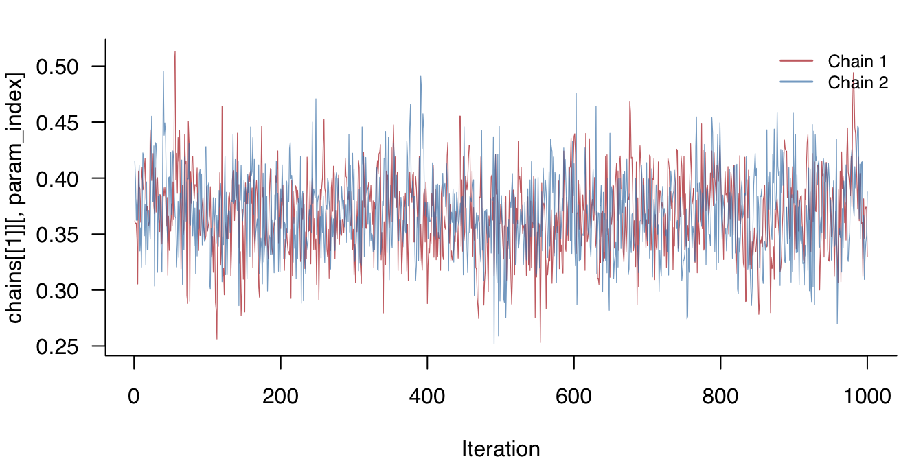
Visually inspecting the sampled values across iterations is a direct way to assess convergence. Chains that have converged look like random noise fluctuating around a stable mean; chains that have not converged show trends, level shifts, or poor mixing.

Raw samples are accessible through fit$raw_samples. The examples on this page use a model fitted to the Wenchuan dataset (17 PTSD symptom items, 362 respondents):

library(bgms)
fit = bgm(Wenchuan, chains = 2, seed = 1234)

param_index = 1
chains = fit$raw_samples$pairwise
nchains = length(chains)
cols = adjustcolor(c("#B22222", "#4682B4", "#2E8B57", "#DAA520"), alpha.f = 0.7)

par(mar = c(4, 4, 1.5, 1), family = "sans")
plot(chains[[1]][, param_index], type = "l", col = cols[1], lwd = 0.6,
  xlab = "Iteration", ylab = colnames(chains[[1]])[param_index],
  ylim = range(sapply(chains, function(ch) range(ch[, param_index]))),
  las = 1, bty = "l")
if(nchains > 1) {
  for(c in 2:nchains) {
    lines(chains[[c]][, param_index], col = cols[c], lwd = 0.6)
  }
}
legend("topright", legend = paste("Chain", seq_len(nchains)),
  col = cols[seq_len(nchains)], lwd = 1.5, bty = "n", cex = 0.8)

Figure 1: Trace plot for the first pairwise interaction parameter across two chains.

NUTS-specific diagnostics

When using update_method = "nuts" (the default), additional diagnostics are stored in fit$nuts_diag.

E-BFMI

E-BFMI (Energy Bayesian Fraction of Missing Information) measures how efficiently the sampler explores the posterior (Betancourt, 2016). It compares the typical size of energy changes between successive samples to the overall spread of energies. Values close to 1 indicate efficient exploration; values below 0.3 suggest the sampler may be getting stuck (Betancourt, 2017).

A low E-BFMI does not necessarily mean the results are wrong, but it does warrant investigation. In models with edge selection, the most common cause is that the warmup period was too short for the discrete graph structure to equilibrate. Increasing warmup often resolves this.

Divergent transitions

Divergent transitions occur when the numerical integrator encounters regions where the posterior curvature changes too rapidly for the current step size. A small number of divergences (fewer than 0.1% of samples) is generally acceptable. Many divergences indicate that the sampler may be missing important parts of the posterior.

If divergences are frequent, increase target_accept (which reduces the step size). If that does not help, try update_method = "adaptive-metropolis" and compare results.

Tree depth

NUTS builds trajectories by repeatedly doubling their length until a U-turn criterion is satisfied. If the trajectory frequently reaches the maximum allowed depth (nuts_max_depth), the sampler may benefit from longer trajectories. Hitting the maximum depth occasionally is normal; hitting it on most iterations may indicate challenging posterior geometry. Consider increasing nuts_max_depth.

Non-reversible steps

For models with continuous variables and edge selection, the leapfrog integrator enforces zero constraints through a projection step (the RATTLE scheme). After each forward step, the integrator checks whether reversing the step returns to the starting point. When the round-trip error exceeds a tolerance scaled by the square of the step size, the step is flagged as non-reversible.

A small number of non-reversible steps is not a concern. A large number indicates that the step size is too large for the constraint geometry. Because the step size is tuned during warmup, the most effective remedy is to increase warmup so the adapter has more time to find an appropriate step size. If non-reversible steps persist after increasing warmup, switch to update_method = "adaptive-metropolis".

Warmup equilibration check

In models with edge selection, the discrete graph structure may take longer to reach stationarity than the continuous parameters. Even after warmup completes, the first portion of the sampling phase may still show transient behavior.

The fit$nuts_diag$warmup_check component provides diagnostics comparing the first and second halves of the post-warmup samples:

Field	Meaning
`warmup_incomplete`	`TRUE` if any indicator below suggests non-stationarity
`energy_slope`	Slope of energy vs. iteration; near zero = stable
`slope_significant`	`TRUE` if energy slope is significant (p < 0.01)
`ebfmi_first_half`	E-BFMI for the first half of post-warmup samples
`ebfmi_second_half`	E-BFMI for the second half
`var_ratio`	Ratio of energy variance (first half / second half); > 2 suggests settling

If these diagnostics suggest the chain was still settling, increase warmup and refit. If diagnostics remain problematic after doubling or tripling warmup, try refitting with update_method = "adaptive-metropolis" and compare posterior summaries. If the two samplers produce similar results, the estimates are likely trustworthy despite the warnings; if they differ, further investigation is warranted.

Recommended workflow

Inspect summary(): check R-hat (< 1.01) and ESS (≥ 100) for all parameters.
Check NUTS diagnostics: fit$nuts_diag$summary for divergences, non-reversible steps, tree depth saturation, and E-BFMI.
Check warmup: fit$nuts_diag$warmup_check for signs of incomplete equilibration.
Plot traces: visually inspect a few key parameters for mixing and stationarity.
If problems are found: increase warmup and/or iter, adjust target_accept, or switch samplers.

References

Betancourt, M. (2016). Diagnosing suboptimal cotangent disintegrations in Hamiltonian Monte Carlo. arXiv Preprint. https://arxiv.org/abs/1604.00695

Betancourt, M. (2017). A conceptual introduction to Hamiltonian Monte Carlo. arXiv Preprint. https://arxiv.org/abs/1701.02434

Gelman, A., & Rubin, D. B. (1992). Inference from iterative simulation using multiple sequences. Statistical Science, 7(4), 457–472. https://doi.org/10.1214/ss/1177011136

Margossian, C. C., & Gelman, A. (2024). For how many iterations should we run Markov chain Monte Carlo? arXiv Preprint. https://doi.org/10.48550/arXiv.2311.02726

van den Bergh, D., Clyde, M. A., Raftery, A. E., & Marsman, M. (2026). Reversible jump MCMC with no regrets: Bayesian variable selection using mixtures of mutually singular distributions. Manuscript in Preparation.

Vehtari, A., Gelman, A., Simpson, D., Carpenter, B., & Bürkner, P.-C. (2021). Rank-normalization, folding, and localization: An improved $\widehat{R}$ for assessing convergence of MCMC (with discussion). Bayesian Analysis, 16(2), 667–718. https://doi.org/10.1214/20-BA1221