Model Output

bgms uses Markov chain Monte Carlo (MCMC) to sample from the posterior distribution of the model parameters. The output of bgm() and bgmCompare() contains posterior summaries computed from these samples, posterior mean matrices, the raw MCMC draws themselves, and sampler diagnostics. This chapter describes how to access and interpret each of these components. For diagnostics related to the sampler itself, see MCMC Diagnostics.

The examples use a fit to the Wenchuan earthquake data (17 ordinal PTSD items):

library(bgms)
fit = bgm(Wenchuan, chains = 2, seed = 1234)

The fit object

bgm() returns a list of class "bgms".

names(fit)

 [1] "posterior_summary_main"      "posterior_summary_pairwise" 
 [3] "posterior_summary_indicator" "posterior_mean_main"        
 [5] "posterior_mean_associations" "posterior_mean_indicator"   
 [7] "arguments"                   "raw_samples"                
 [9] "nuts_diag"                   ".bgm_spec"

The two primary interfaces are summary() for tabular diagnostics and coef() for posterior means in matrix form. Raw samples are available in fit$raw_samples for custom analyses.

Posterior summaries

Calling summary() prints formatted tables of posterior statistics.

summary(fit)

Posterior summaries from Bayesian estimation:

Category thresholds: 
                 mean  mcse    sd   n_eff  Rhat
intrusion (1)   0.457 0.010 0.250 580.592 1.009
intrusion (2)  -2.035 0.024 0.387 259.263 1.006
intrusion (3)  -5.276 0.045 0.661 214.646 1.006
intrusion (4) -10.347 0.066 1.038 248.274 1.003
dreams (1)     -0.817 0.008 0.212 675.187 1.000
dreams (2)     -4.379 0.020 0.420 436.475 1.001
... (use `summary(fit)$main` to see full output)

Pairwise interactions:
                    mean    sd  mcse   n_eff  Rhat
intrusion-dreams   0.369 0.001 0.037 848.100 1.000
intrusion-flash    0.165 0.001 0.034 623.634 1.055
intrusion-upset    0.062 0.055 0.008  46.612 1.058
intrusion-physior  0.007 0.020 0.002 151.748 1.000
intrusion-avoidth  0.000 0.000 0.000  84.121 1.000
intrusion-avoidact 0.000 0.001 0.000 146.722 1.000
... (use `summary(fit)$pairwise` to see full output)
Note: NA values are suppressed in the print table. They occur here when an 
indicator was zero across all iterations, so mcse/n_eff/n_eff_mixt/Rhat are undefined;
`summary(fit)$pairwise` still contains the NA values.

Inclusion probabilities:
                    mean    sd  mcse n0->0 n0->1 n1->0 n1->1    n_eff  Rhat
intrusion-dreams   1.000 0.000           0     0     0  1999               
intrusion-flash    1.000 0.000           0     0     0  1999               
intrusion-upset    0.599 0.490 0.076   781    19    20  1179   41.265 1.116
intrusion-physior  0.106 0.308 0.025  1760    27    27   185  153.394     1
intrusion-avoidth  0.008 0.089 0.002  1969    14    14     2  1578.01  1.03
intrusion-avoidact 0.012 0.109 0.003  1957    18    18     6 1223.503  1.03
... (use `summary(fit)$indicator` to see full output)
Note: NA values are suppressed in the print table. They occur when an indicator
was constant or had fewer than 5 transitions, so n_eff_mixt is unreliable;
`summary(fit)$indicator` still contains all computed values.

Use `summary(fit)$<component>` to access full results.
Use `extract_log_odds(fit)` for log odds ratios.
See the `easybgm` package for other summary and plotting tools.

Reading the output

The summary produces a set of tables depending on the model type. Each row is a parameter; each column is a posterior summary statistic. The tables that appear depend on which model was fitted:

Table	OMRF	GGM	Mixed MRF
Category thresholds	yes	—	yes (discrete block)
Continuous means	—	—	yes (continuous block)
Residual variances	—	yes	yes (continuous block)
Pairwise interactions	yes	yes	yes
Inclusion indicators	if edge selection	if edge selection	if edge selection

Category thresholds report the posterior estimates of the ordinal threshold parameters. These define the boundary between adjacent response categories on the log-odds scale. Negative values indicate that higher categories are less probable.

Residual variances report the posterior estimates of the residual variance $1 / \Theta_{ii}$ for each continuous variable, where $\Theta_{ii}$ is the corresponding diagonal element of the precision matrix. Use extract_precision() to obtain the full precision matrix.

Pairwise interactions report the conditional association between each pair of variables, controlling for all others. These are the edge weights in the graphical model. A value of zero means the two variables are conditionally independent. For mixed models, these span three blocks: discrete–discrete, continuous–continuous, and cross-type edges. Use extract_partial_correlations() for standardized partial correlations (continuous variables) and extract_log_odds() for log-odds ratios (discrete variables).

Inclusion indicators report the posterior inclusion probability of each edge. An inclusion probability near 1 indicates strong evidence for the edge; near 0 indicates strong evidence against it. Values around 0.5 are inconclusive. The transition counts (n0->0, n0->1, n1->0, n1->1) show how often the edge indicator switched between excluded (0) and included (1) states during sampling. Edges with very few transitions (fewer than 5) have unreliable mixture ESS estimates; bgms suppresses these automatically.

Summary columns

Column	Meaning
`mean`	Posterior mean of the parameter.
`sd`	Posterior standard deviation — the width of the posterior.
`mcse`	Monte Carlo standard error — how precisely the posterior mean is estimated. A small MCSE relative to `sd` indicates sufficient sampling. See MCMC Diagnostics.
`n_eff`	Effective sample size — the number of independent draws the chain is equivalent to. Values below 100 warrant longer runs. See MCMC Diagnostics.
`n_eff_mixt`	Mixture ESS for binary edge indicators, accounting for the spike-and-slab structure. See MCMC Diagnostics.
`Rhat`	Split $\hat{R}$ convergence diagnostic. Values above 1.01 suggest the chains have not mixed. See MCMC Diagnostics.

Accessing specific tables

The printed output is truncated. Access the full tables with:

head(summary(fit)$main, 4)

                     mean       mcse        sd    n_eff     Rhat
intrusion (1)   0.4568169 0.01038543 0.2502419 580.5918 1.009444
intrusion (2)  -2.0354043 0.02402363 0.3868202 259.2634 1.005916
intrusion (3)  -5.2762183 0.04511390 0.6609543 214.6457 1.006201
intrusion (4) -10.3474787 0.06588472 1.0381272 248.2743 1.002817

head(summary(fit)$pairwise, 4)

                         mean          sd        mcse     n_eff      Rhat
intrusion-dreams  0.368601582 0.001253424 0.036502412 848.09972 0.9998857
intrusion-flash   0.165474538 0.001380939 0.034485738 623.63446 1.0553821
intrusion-upset   0.062490783 0.055032261 0.008060624  46.61197 1.0576230
intrusion-physior 0.006943673 0.020399916 0.001656027 151.74757 0.9997753

head(summary(fit)$indicator, 4)

                    mean        sd       mcse n0->0 n0->1 n1->0 n1->1     n_eff
intrusion-dreams  1.0000 0.0000000         NA     0     0     0  1999        NA
intrusion-flash   1.0000 0.0000000         NA     0     0     0  1999        NA
intrusion-upset   0.5995 0.4899997 0.07627922   781    19    20  1179  41.26475
intrusion-physior 0.1060 0.3078376 0.02485517  1760    27    27   185 153.39448
                       Rhat
intrusion-dreams         NA
intrusion-flash          NA
intrusion-upset   1.1160963
intrusion-physior 0.9997014

Posterior mean matrices

The coef() method returns posterior means in matrix form — convenient for network visualization and downstream analysis.

str(coef(fit), max.level = 1)

List of 3
 $ main     : num [1:17, 1:4] 0.4568 -0.8175 -0.3684 0.0698 -0.6866 ...
  ..- attr(*, "dimnames")=List of 2
 $ pairwise : num [1:17, 1:17] 0 0.3686 0.16547 0.06249 0.00694 ...
  ..- attr(*, "dimnames")=List of 2
 $ indicator: num [1:17, 1:17] 0 1 1 0.599 0.106 ...
  ..- attr(*, "dimnames")=List of 2

coef(fit)$pairwise is a symmetric $p \times p$ matrix of posterior mean partial associations (zero diagonal). For interpretable scales, use extract_precision(), extract_partial_correlations(), or extract_log_odds(). coef(fit)$indicator is a symmetric $p \times p$ matrix of posterior inclusion probabilities.

For ordinal models, coef(fit)$main is a matrix with variables in rows and category thresholds in columns:

coef(fit)$main[1:4, ]

              cat (1)   cat (2)   cat (3)   cat (4)
intrusion  0.45681686 -2.035404 -5.276218 -10.34748
dreams    -0.81747952 -4.379279 -8.213524 -13.31259
flash     -0.36844405 -3.228067 -6.626082 -11.70289
upset      0.06981198 -2.197320 -5.173231 -10.07425

Raw MCMC samples

For custom analyses — posterior intervals, density plots, or derived quantities — the raw posterior draws are stored in fit$raw_samples:

str(fit$raw_samples, max.level = 1)

List of 7
 $ main           :List of 2
 $ pairwise       :List of 2
 $ indicator      :List of 2
 $ allocations    : NULL
 $ nchains        : int 2
 $ niter          : int 1000
 $ parameter_names:List of 4

Each element is a list of matrices, one per chain, with rows = iterations and columns = parameters. The chains are stored separately to allow per-chain diagnostics.

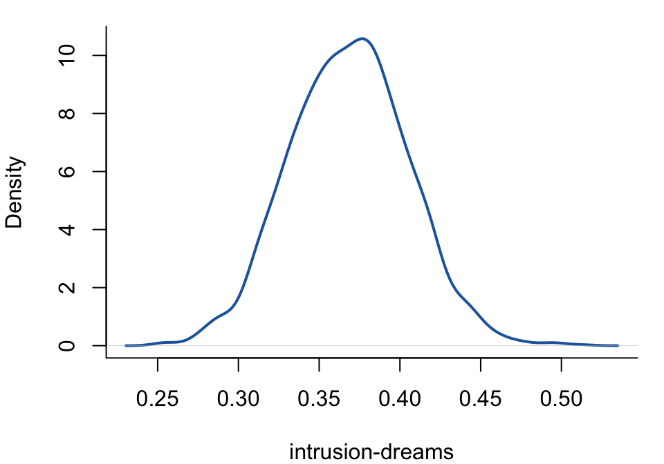
Example: posterior density for an edge

To extract the posterior samples for the intrusion–dreams interaction and compute a 95% credible interval:

# Combine chains for one parameter
edge = "intrusion-dreams"
col_idx = which(fit$raw_samples$parameter_names$pairwise == edge)
samples_c1 = fit$raw_samples$pairwise[[1]][, col_idx]
samples_c2 = fit$raw_samples$pairwise[[2]][, col_idx]
samples = c(samples_c1, samples_c2)

cat("Posterior mean:", round(mean(samples), 3), "\n")

Posterior mean: 0.369

cat("95% CI: [", round(quantile(samples, 0.025), 3), ",",
    round(quantile(samples, 0.975), 3), "]\n")

95% CI: [ 0.299 , 0.44 ]

par(mar = c(4, 4, 1, 1))
plot(density(samples), main = "", xlab = "intrusion-dreams",
  ylab = "Density", bty = "L", lwd = 2, col = "#2166AC")
abline(v = 0, lty = 2, col = "grey50")

Extracting specific results

The extract_*() family of functions provides targeted access to model components. These are documented in the Extractor Functions reference. The most commonly used are:

Function	Returns
`extract_pairwise_interactions()`	Raw partial association samples
`extract_main_effects()`	Raw main effect samples
`extract_indicators()`	Raw indicator samples
`extract_posterior_inclusion_probabilities()`	Posterior inclusion probabilities
`extract_precision()`	Posterior mean precision matrix (GGM / continuous block)
`extract_partial_correlations()`	Posterior mean partial correlation matrix (GGM / continuous block)
`extract_log_odds()`	Posterior mean log-odds matrix (ordinal / discrete block)
`extract_ess()`	Effective sample sizes
`extract_rhat()`	Split $\hat{R}$ values
`extract_sbm()`	SBM cluster assignments and co-clustering matrix (when `edge_prior = "Stochastic-Block"`)
`extract_arguments()`	Arguments used when fitting the model

NUTS diagnostics

When update_method = "nuts" (the default), additional diagnostics are stored in fit$nuts_diag:

str(fit$nuts_diag, max.level = 1)

List of 6
 $ treedepth   : num [1:2, 1:1000] 5 4 5 5 5 5 4 5 5 5 ...
 $ divergent   : num [1:2, 1:1000] 0 0 0 0 0 0 0 0 0 0 ...
 $ energy      : num [1:2, 1:1000] 6684 6654 6673 6663 6681 ...
 $ ebfmi       : num [1:2] 0.746 0.77
 $ warmup_check:List of 6
 $ summary     :List of 4

The summary field contains per-chain summaries of tree depth, divergences, non-reversible steps, and energy. The warmup_check field reports whether warmup equilibration was sufficient. These are described in detail in MCMC Diagnostics. If these diagnostics remain problematic after tuning, refit with update_method = "adaptive-metropolis".

Output from `bgmCompare()`

bgmCompare() returns a list of class "bgmCompare" with the same structure as bgm(), plus additional components for group differences. The examples use the ADHD data (18 binary items, two groups):

fit_compare = bgmCompare(
  x = ADHD[, -1],
  group_indicator = ADHD$group,
  variable_type = "ordinal",
  chains = 2,
  seed = 1234
)

summary(fit_compare)

Posterior summaries from Bayesian grouped MRF estimation (bgmCompare):

Category thresholds:
     parameter   mean  mcse    sd    n_eff  Rhat
1    avoid (1) -3.408 0.021 0.608  826.759 1.000
2 closeatt (1) -2.771 0.017 0.543 1067.896 1.002
3 distract (1) -2.359 0.021 0.546  647.922 1.015
4   forget (1) -2.234 0.018 0.549  931.707 1.002
5 instruct (1) -3.555 0.023 0.665  816.265 1.001
6   listen (1) -1.331 0.026 0.651  651.067 1.008
... (use `summary(fit)$main` to see full output)

Pairwise interactions:
       parameter   mean  mcse    sd    n_eff  Rhat
1 avoid-closeatt  1.083 0.020 0.512  625.405 1.001
2 avoid-distract  1.892 0.011 0.389 1353.472 1.002
3   avoid-forget  0.703 0.015 0.420  734.835 1.002
4 avoid-instruct  1.063 0.025 0.535  469.108 1.002
5   avoid-listen -0.149 0.015 0.477 1041.748 1.000
6    avoid-loses  0.216 0.012 0.398 1189.310 1.003
... (use `summary(fit)$pairwise` to see full output)

Inclusion probabilities:
                 parameter  mean    sd  mcse n0->0 n0->1 n1->0 n1->1    n_eff
              avoid (main) 1.000 0.000           0     0     0  1999         
 avoid-closeatt (pairwise) 0.843 0.363 0.014   185   128   128  1558  640.029
 avoid-distract (pairwise) 0.382 0.486 0.012   809   426   425   339 1640.408
   avoid-forget (pairwise) 0.798 0.401 0.017   259   145   145  1450  580.345
 avoid-instruct (pairwise) 0.914 0.281 0.012   102    71    71  1755  579.459
   avoid-listen (pairwise) 0.659 0.474 0.017   421   261   261  1056  818.639
  Rhat
      
 1.001
     1
 1.002
 1.022
     1
... (use `summary(fit)$indicator` to see full output)
Note: NA values are suppressed in the print table. They occur when an indicator
was constant or had fewer than 5 transitions, so n_eff_mixt is unreliable;
`summary(fit)$indicator` still contains all computed values.

Group differences (main effects):
           parameter  mean    sd mcse n_eff  Rhat
    avoid (diff1; 1) 1.763 1.146            1.005
 closeatt (diff1; 1) 2.656 1.090            1.003
 distract (diff1; 1) 0.519 0.965            1.009
   forget (diff1; 1) 2.274 1.022            1.004
 instruct (diff1; 1) 1.601 1.257            1.001
   listen (diff1; 1) 3.921 1.310            1.000
... (use `summary(fit)$main_diff` to see full output)
Note: NA values are suppressed in the print table. They occur here when an
indicator was zero across all iterations, so mcse/n_eff/n_eff_mixt/Rhat are undefined;
`summary(fit)$main_diff` still contains the NA values.

Group differences (pairwise effects):
              parameter   mean    sd  mcse   n_eff  Rhat
 avoid-closeatt (diff1) -1.545 1.039 0.040 688.378 1.000
 avoid-distract (diff1) -0.212 0.373 0.015 592.635 1.000
   avoid-forget (diff1) -1.188 0.865 0.036 588.020 1.002
 avoid-instruct (diff1)  2.179 1.215 0.052 545.404 1.000
   avoid-listen (diff1)  0.922 0.932 0.038 613.600 1.000
    avoid-loses (diff1) -0.303 0.467 0.015 955.778 1.000
... (use `summary(fit)$pairwise_diff` to see full output)
Note: NA values are suppressed in the print table. They occur here when an
indicator was zero across all iterations, so mcse/n_eff/n_eff_mixt/Rhat are undefined;
`summary(fit)$pairwise_diff` still contains the NA values.

Use `summary(fit)$<component>` to access full results.
See the `easybgm` package for other summary and plotting tools.

The summary includes two additional tables beyond what bgm() produces:

Group differences (main effects) — posterior estimates of how category thresholds differ between the two groups. Large positive or negative values indicate that a symptom’s baseline severity differs across groups.
Group differences (pairwise effects) — posterior estimates of how edge weights differ between the two groups. These quantify whether the conditional association between two symptoms is stronger or weaker in one group relative to the other.

When difference_selection = TRUE (the default), the inclusion indicators for these difference parameters are reported alongside the common-structure indicators. An inclusion probability near 1 for a difference parameter indicates strong evidence that the groups differ on that effect.