Diagnostics and Spike-and-Slab Summaries • bgms

Introduction

This vignette illustrates how to inspect convergence diagnostics and how to interpret spike-and-slab summaries in bgms models. For some of the model variables spike-and-slab priors introduce binary indicator variables that govern whether the effect is included or not. Their posterior distributions can be summarized with inclusion probabilities and Bayes factors.

Example fit

We use a subset of the Wenchuan dataset:

library(bgms)
data = Wenchuan[, 1:5]
fit = bgm(data, seed = 1234)

Convergence diagnostics

The quality of the Markov chain can be assessed with common MCMC diagnostics:

summary(fit)$pairwise
#>                          mean         mcse          sd     n_eff
#> intrusion-dreams  0.316707142 0.0010098545 0.034591884 1173.3587
#> intrusion-flash   0.167709696 0.0009227124 0.032098600 1210.1506
#> intrusion-upset   0.088672349 0.0056294194 0.043688239  101.0666
#> intrusion-physior 0.101880020 0.0024784801 0.033795461  361.6609
#> dreams-flash      0.249884872 0.0008231779 0.030402369 1364.0412
#> dreams-upset      0.118073148 0.0013525831 0.027885151  425.0286
#> dreams-physior    0.001072865 0.0003205022 0.006603434  484.5981
#> flash-upset       0.001168627 0.0004414651 0.007661098 2935.6176
#> flash-physior     0.152192873 0.0007852046 0.027777015 1251.4270
#> upset-physior     0.355534822 0.0008746934 0.032272128 1361.2675
#>                   n_eff_mixt     Rhat
#> intrusion-dreams          NA 1.003034
#> intrusion-flash           NA 1.004751
#> intrusion-upset     60.22847 1.047652
#> intrusion-physior  185.92847 1.030492
#> dreams-flash              NA 1.002973
#> dreams-upset              NA 1.003959
#> dreams-physior     424.49999 1.008677
#> flash-upset        301.15450 1.297113
#> flash-physior             NA 1.001141
#> upset-physior             NA 1.005101

R-hat values close to 1 (typically below 1.01) suggest convergence (Vehtari et al., 2021).
The effective sample size (ESS) reflects the number of independent samples that would provide equivalent precision. Larger ESS values indicate more reliable estimates.
The Monte Carlo standard error (MCSE) measures the additional variability introduced by using a finite number of MCMC draws. A small MCSE relative to the posterior standard deviation indicates stable estimates, whereas a large MCSE suggests that more samples are needed.

Two ESS measures for edge-selected parameters

With edge or difference selection active, the effect parameters are governed by spike-and-slab priors. The corresponding parameter is set to exactly zero when the effect is excluded, rather than being removed from the model. Because the parameter has a well-defined value at every iteration, the full chain — including zeros — is a valid sequence for computing ESS.

n_eff is the unconditional ESS, computed from the full effect chain. It measures how precisely the overall posterior mean is estimated.
n_eff_mixt is the mixture ESS. It measures how precisely the posterior mean of the effect is estimated while accounting for the additional uncertainty introduced by the spike-and-slab selection. When the indicator rarely switches between inclusion and exclusion (fewer than 5 transitions), n_eff_mixt is suppressed in the printed output.

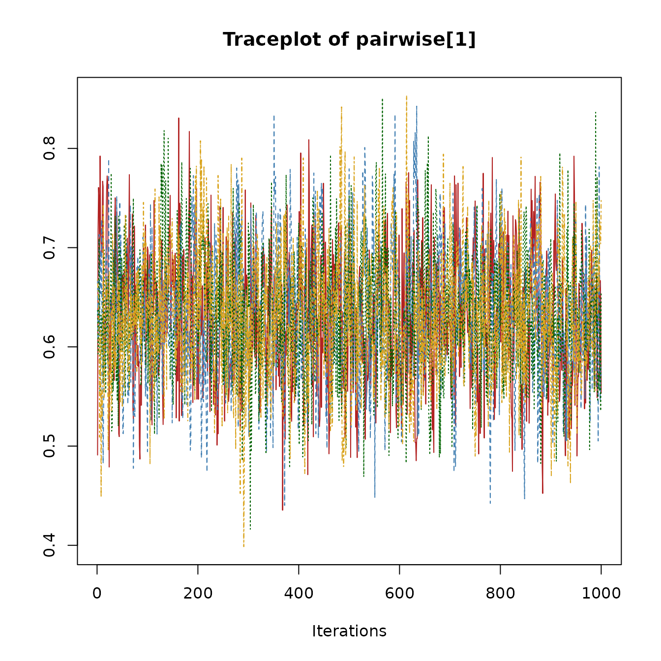
Traceplots

Users can inspect traceplots by extracting raw samples directly. Here is an example for the pairwise effect parameter.

param_index = 1
chains = fit$raw_samples$pairwise
nchains = length(chains)
cols = c("firebrick", "steelblue", "darkgreen", "goldenrod")

plot(chains[[1]][, param_index], type = "l", col = cols[1],
  xlab = "Iteration", ylab = "Value",
  main = "Traceplot of pairwise[1]",
  ylim = range(sapply(chains, function(ch) range(ch[, param_index]))))
if(nchains > 1) {
  for(c in 2:nchains) {
    lines(chains[[c]][, param_index], col = cols[c])
  }
}

Spike-and-slab summaries

The spike-and-slab prior yields posterior inclusion probabilities for edges:

coef(fit)$indicator
#>           intrusion dreams flash  upset physior
#> intrusion    0.0000  1.000 1.000 0.8645  0.9705
#> dreams       1.0000  0.000 1.000 1.0000  0.0260
#> flash        1.0000  1.000 0.000 0.0230  1.0000
#> upset        0.8645  1.000 0.023 0.0000  1.0000
#> physior      0.9705  0.026 1.000 1.0000  0.0000

Values near 1.0: strong evidence the edge is present.
Values near 0.0: strong evidence the edge is absent.
Values near 0.5: inconclusive (absence of evidence).

Bayes factors

When the prior inclusion probability for an edge is equal to 0.5 (e.g., using a Bernoulli prior with inclusion_probability = 0.5 or a symmetric Beta prior, main_alpha = main_beta), we can directly transform inclusion probabilities into Bayes factors for edge presence vs absence:

# Example for one edge
p = coef(fit)$indicator[1, 5]
BF_10 = p / (1 - p)
BF_10
#> [1] 32.89831

Here the Bayes factor in favor of inclusion (H1) is small, meaning that there is little evidence for inclusion. Since the Bayes factor is transitive, we can use it to express the evidence in favor of exclusion (H0) as

1 / BF_10
#> [1] 0.0303967

This Bayes factor shows that there is strong evidence for the absence of a network relation between the variables intrusion and physior.

NUTS diagnostics

When using update_method = "nuts" (the default), additional diagnostics are available to assess the quality of the Hamiltonian Monte Carlo sampling. These can be accessed via fit$nuts_diag:

fit$nuts_diag$summary
#> $total_divergences
#> [1] 0
#> 
#> $max_tree_depth_hits
#> [1] 0
#> 
#> $min_ebfmi
#> [1] 0.9414881
#> 
#> $warmup_incomplete
#> [1] TRUE

E-BFMI

E-BFMI (Energy Bayesian Fraction of Missing Information) measures how efficiently the sampler explores the posterior. It compares the typical size of energy changes between successive samples to the overall spread of energies. Values close to 1 indicate that the sampler moves freely across the energy landscape; values below 0.3 suggest the sampler may be getting stuck or that the chain has not yet settled into its stationary distribution.

A low E-BFMI does not necessarily mean your results are wrong, but it does warrant further investigation. In models with edge selection, the most common cause is that the warmup period was too short for the discrete graph structure to equilibrate. Increasing warmup often resolves this.

Divergent transitions

Divergent transitions occur when the numerical integrator encounters regions of the posterior where the curvature changes too rapidly for the current step size. A small number of divergences (say, fewer than 0.1% of samples) is generally acceptable. However, many divergences indicate that the sampler may be missing important parts of the posterior.

If you see a large number of divergences, consider increasing target_accept (which makes the sampler use a smaller step size) and, if this does not fix it, switching to update_method = "adaptive-metropolis".

Tree depth

NUTS builds trajectories by repeatedly doubling their length until a “U-turn” criterion is satisfied. If the trajectory frequently reaches the maximum allowed depth (nuts_max_depth, default 10), it suggests the sampler may benefit from longer trajectories to explore the posterior efficiently. Hitting the maximum depth occasionally is normal; hitting it on most iterations may indicate challenging posterior geometry. If this happens, consider increasing nuts_max_depth.

Warmup and equilibration

Standard HMC/NUTS warmup is designed to tune the step size and mass matrix for the continuous parameters. In models with edge selection, the discrete graph structure may take longer to reach its stationary distribution than the continuous parameters. As a result, even after warmup completes, the first portion of the sampling phase may still show transient behavior (i.e., non-stationarity).

The warmup_check component provides simple diagnostics that compare the first and second halves of the post-warmup samples:

fit$nuts_diag$warmup_check
#> $warmup_incomplete
#> [1] TRUE TRUE
#> 
#> $energy_slope
#>     time_idx     time_idx 
#> -0.001635190  0.004198063 
#> 
#> $slope_significant
#> time_idx time_idx 
#>     TRUE     TRUE 
#> 
#> $ebfmi_first_half
#> [1] 0.9586055 0.9940538
#> 
#> $ebfmi_second_half
#> [1] 0.9304157 0.9690688
#> 
#> $var_ratio
#> [1] 1.0693025 0.9312399

The returned list contains the following fields (one value per chain):

warmup_incomplete: A logical flag that is TRUE when any of the indicators below suggest the chain may not have reached stationarity.
energy_slope: The slope of a linear regression of energy against iteration number. A slope near zero indicates stable energy; a significant negative slope suggests the chain is still drifting toward higher-probability regions.
slope_significant: TRUE if the energy slope is statistically significant (p < 0.01).
ebfmi_first_half and ebfmi_second_half: E-BFMI computed separately for the first and second halves of the post-warmup samples. If the first-half value is much lower (for example, below 0.3) while the second-half value is healthy, the early samples were likely still settling.
var_ratio: The ratio of energy variance in the first half to that in the second half. A ratio much greater than 1 (for example, above 2) indicates higher variability early on, consistent with transient behavior.

If these diagnostics suggest the chain was still settling, increase warmup and re-run the model. If diagnostics remain problematic after a substantial increase (for example, doubling or tripling warmup), consider re-fitting with update_method = "adaptive-metropolis" and comparing the posterior summaries. If the two samplers produce similar results, the estimates are likely trustworthy despite the warnings; if they differ substantially, that warrants further investigation of the model or data.

Next steps

See Getting Started for a simple one-sample workflow.
See Model Comparison for group differences.

Vehtari, A., Gelman, A., Simpson, D., Carpenter, B., & Bürkner, P.-C. (2021). Rank-normalization, folding, and localization: An improved

\hat{R}

for assessing convergence of MCMC. Bayesian Analysis, 16(2), 667–718. https://doi.org/10.1214/20-BA1221