Introduction
The function bgmCompare() extends bgm() to
independent-sample designs. It estimates whether edge weights and
category thresholds differ across groups in an ordinal Markov random
field (MRF).
Posterior inclusion probabilities indicate how plausible it is that a group difference exists in a given parameter. These can be converted to Bayes factors for hypothesis testing.
Fitting a model
fit = bgmCompare(x = data_adhd, y = data_no_adhd, seed = 1234)Posterior summaries
The summary shows both baseline effects and group differences:
summary(fit)
#> Posterior summaries from Bayesian grouped MRF estimation (bgmCompare):
#>
#> Category thresholds:
#>      parameter   mean  mcse    sd    n_eff  Rhat
#> 1    avoid (1) -2.594 0.006 0.369 3904.974 1.000
#> 2 closeatt (1) -2.231 0.006 0.358 4153.680 1.001
#> 3 distract (1) -0.438 0.006 0.321 2504.279 1.000
#> 4   forget (1) -1.546 0.005 0.314 4216.099 1.000
#> 5 instruct (1) -2.318 0.008 0.394 2542.043 1.000
#>
#> Pairwise interactions:
#>           parameter   mean  mcse    sd    n_eff  Rhat
#> 1    avoid-closeatt  0.824 0.010 0.451 2211.995 1.001
#> 2    avoid-distract  1.642 0.005 0.353 4490.559 1.000
#> 3      avoid-forget  0.474 0.007 0.360 2725.903 1.000
#> 4    avoid-instruct  0.365 0.007 0.422 3365.540 1.001
#> 5 closeatt-distract -0.180 0.006 0.358 4141.167 1.001
#> 6   closeatt-forget  0.134 0.004 0.280 4026.262 1.001
#> ... (use `summary(fit)$pairwise` to see full output)
#>
#> Inclusion probabilities:
#>                  parameter  mean  mcse    sd n0->0 n0->1 n1->0 n1->1
#>               avoid (main) 1.000       0.000     0     0     0  3999
#>  avoid-closeatt (pairwise) 0.713 0.013 0.453   757   393   393  2456
#>  avoid-distract (pairwise) 0.400 0.008 0.490  1497   905   905   692
#>    avoid-forget (pairwise) 0.828 0.011 0.377   437   251   251  3060
#>  avoid-instruct (pairwise) 0.997 0.001 0.052     5     6     6  3982
#>            closeatt (main) 1.000       0.000     0     0     0  3999
#>  n_eff_mixt  Rhat
#>
#>    1262.058     1
#>    3571.863     1
#>    1130.288 1.004
#>    1505.695 1.004
#>
#> ... (use `summary(fit)$indicator` to see full output)
#> Note: NA values are suppressed in the print table. They occur when an indicator
#> was constant or had fewer than 5 transitions, so n_eff_mixt is unreliable;
#> `summary(fit)$indicator` still contains all computed values.
#>
#> Group differences (main effects):
#>            parameter   mean mcse    sd    n_eff n_eff_mixt  Rhat
#>     avoid (diff1; 1) -2.536      0.720 3215.273            1.000
#>  closeatt (diff1; 1) -2.947      0.715 3515.888            1.000
#>  distract (diff1; 1) -2.620      0.656 2188.558            1.002
#>    forget (diff1; 1) -2.869      0.647 2976.872            1.000
#>  instruct (diff1; 1) -2.451      0.870 1786.664            1.000
#> Note: NA values are suppressed in the print table. They occur here when an
#> indicator was zero across all iterations, so mcse/n_eff/n_eff_mixt/Rhat are undefined;
#> `summary(fit)$main_diff` still contains the NA values.
#>
#> Group differences (pairwise effects):
#>                  parameter   mean  mcse    sd    n_eff n_eff_mixt
#>     avoid-closeatt (diff1)  1.001 0.021 0.867 1567.759   1656.744
#>     avoid-distract (diff1)  0.212 0.007 0.349 2987.491   2466.120
#>       avoid-forget (diff1)  1.212 0.019 0.806 1706.692   1738.038
#>     avoid-instruct (diff1) -2.791 0.018 0.957 2732.896   2807.830
#>  closeatt-distract (diff1) -0.148 0.008 0.305 2838.680   1542.273
#>    closeatt-forget (diff1)  0.158 0.007 0.309 2836.020   1810.940
#>   Rhat
#>  1.000
#>  1.000
#>  1.000
#>  1.002
#>  1.000
#>  1.009
#> ... (use `summary(fit)$pairwise_diff` to see full output)
#> Note: NA values are suppressed in the print table. They occur here when an
#> indicator was zero across all iterations, so mcse/n_eff/n_eff_mixt/Rhat are undefined;
#> `summary(fit)$pairwise_diff` still contains the NA values.
#>
#> Use `summary(fit)$<component>` to access full results.
#> See the `easybgm` package for other summary and plotting tools.
You can extract posterior means and inclusion probabilities:
coef(fit)
#> $main_effects_raw
#>                baseline     diff1
#> avoid(c1)    -2.5938427 -2.536236
#> closeatt(c1) -2.2314062 -2.947048
#> distract(c1) -0.4376243 -2.619701
#> forget(c1)   -1.5461688 -2.868977
#> instruct(c1) -2.3179644 -2.450688
#>
#> $pairwise_effects_raw
#>                     baseline      diff1
#> avoid-closeatt     0.8235010  1.0011702
#> avoid-distract     1.6421831  0.2116882
#> avoid-forget       0.4739962  1.2119262
#> avoid-instruct     0.3651010 -2.7912009
#> closeatt-distract -0.1801949 -0.1475133
#> closeatt-forget    0.1336782  0.1583270
#> closeatt-instruct  1.4962870  0.5472581
#> distract-forget    0.3727393  0.2242070
#> distract-instruct  1.1876278  1.3106551
#> forget-instruct    1.0735725  0.7942729
#>
#> $main_effects_groups
#>                  group1    group2
#> avoid(c1)    -1.3257244 -3.861961
#> closeatt(c1) -0.7578823 -3.704930
#> distract(c1)  0.8722263 -1.747475
#> forget(c1)   -0.1116801 -2.980657
#> instruct(c1) -1.0926202 -3.543309
#>
#> $pairwise_effects_groups
#>                        group1     group2
#> avoid-closeatt     0.32291585  1.3240861
#> avoid-distract     1.53633900  1.7480272
#> avoid-forget      -0.13196684  1.0799593
#> avoid-instruct     1.76070148 -1.0304994
#> closeatt-distract -0.10643820 -0.2539515
#> closeatt-forget    0.05451476  0.2128417
#> closeatt-instruct  1.22265789  1.7699160
#> distract-forget    0.26063585  0.4848428
#> distract-instruct  0.53230029  1.8429554
#> forget-instruct    0.67643605  1.4707089
#>
#> $indicators
#>            avoid closeatt distract  forget instruct
#> avoid    1.00000  0.71250  0.39950 0.82800  0.99725
#> closeatt 0.71250  1.00000  0.35275 0.36950  0.56550
#> distract 0.39950  0.35275  1.00000 0.40025  0.87125
#> forget   0.82800  0.36950  0.40025 1.00000  0.71600
#> instruct 0.99725  0.56550  0.87125 0.71600  1.00000
Visualizing group networks
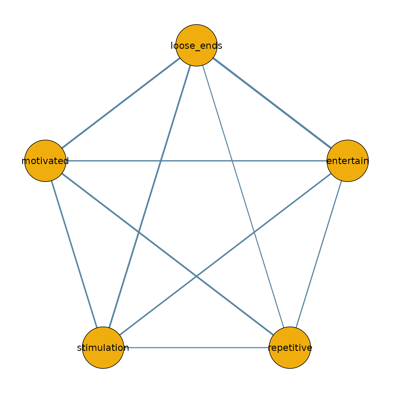
We can use the output to plot the network for the ADHD group:
library(qgraph)

adhd_network = matrix(0, 5, 5)
adhd_network[lower.tri(adhd_network)] = coef(fit)$pairwise_effects_groups[, 1]
adhd_network = adhd_network + t(adhd_network)
colnames(adhd_network) = colnames(data_adhd)
rownames(adhd_network) = colnames(data_adhd)

qgraph(adhd_network,
  theme = "TeamFortress",
  maximum = 1,
  fade = FALSE,
  color = c("#f0ae0e"), vsize = 10, repulsion = .9,
  label.cex = 1, label.scale = "FALSE",
  labels = colnames(data_adhd)
)