Getting Started with bgms • bgms

Introduction

The bgms package implements Bayesian methods for analyzing graphical models. It supports three variable types:

ordinal (including binary) — Markov random field (MRF) models,
Blume–Capel — ordinal MRF with a reference category,
continuous — Gaussian graphical models (GGM).

The package estimates main effects and pairwise interactions, with optional Bayesian edge selection via spike-and-slab priors. It provides two main entry points:

bgm() for one-sample designs (single network),
bgmCompare() for independent-sample designs (group comparisons).

This vignette walks through the basic workflow for ordinal data. For continuous data, set variable_type = "continuous" in bgm() to fit a Gaussian graphical model.

Wenchuan dataset

The dataset Wenchuan contains responses from survivors of the 2008 Wenchuan earthquake on posttraumatic stress items. Here, we analyze a subset of the first five items as a demonstration.

library(bgms)

# Analyse a subset of the Wenchuan dataset
?Wenchuan
data = Wenchuan[, 1:5]
head(data)
#>      intrusion dreams flash upset physior
#> [1,]         2      2     2     2       3
#> [2,]         2      2     2     3       3
#> [3,]         2      4     4     4       3
#> [4,]         2      1     2     2       1
#> [5,]         2      2     2     2       2
#> [6,]         4      3     2     2       2

Fitting a model

The main entry point is bgm() for single-group models and bgmCompare() for multiple-group comparisons.

fit = bgm(data, seed = 1234)

Posterior summaries

summary(fit)
#> Posterior summaries from Bayesian estimation:
#> 
#> Category thresholds:
#>                 mean  mcse    sd   n_eff  Rhat
#> intrusion (1)  0.495 0.009 0.239 773.785 1.000
#> intrusion (2) -1.855 0.017 0.356 466.298 1.001
#> intrusion (3) -4.765 0.034 0.595 306.989 1.003
#> intrusion (4) -9.383 0.051 0.951 343.491 1.002
#> dreams (1)    -0.595 0.006 0.196 950.372 1.009
#> dreams (2)    -3.805 0.013 0.360 784.143 1.014
#> ... (use `summary(fit)$main` to see full output)
#> 
#> Pairwise interactions:
#>                    mean    sd  mcse    n_eff  Rhat
#> intrusion-dreams  0.632 0.002 0.067 1246.221 1.003
#> intrusion-flash   0.338 0.002 0.067 1106.040 1.000
#> intrusion-upset   0.180 0.091 0.011   73.901 1.043
#> intrusion-physior 0.195 0.077 0.007  121.806 1.053
#> dreams-flash      0.501 0.002 0.060 1202.087 1.000
#> dreams-upset      0.233 0.058 0.003  512.733 1.019
#> ... (use `summary(fit)$pairwise` to see full output)
#> Note: NA values are suppressed in the print table. They occur here when an 
#> indicator was zero across all iterations, so mcse/n_eff/Rhat are undefined;
#> `summary(fit)$pairwise` still contains the NA values.
#> 
#> Inclusion probabilities:
#>                    mean    sd  mcse n0->0 n0->1 n1->0 n1->1   n_eff
#> intrusion-dreams  1.000 0.000           0     0     0  1999        
#> intrusion-flash   1.000 0.000           0     0     0  1999        
#> intrusion-upset   0.858 0.350 0.049   273    12    12  1702  50.343
#> intrusion-physior 0.931 0.253  0.03   128     9     9  1853  73.105
#> dreams-flash      1.000 0.000           0     0     0  1999        
#> dreams-upset      0.999 0.039 0.002     2     1     1  1995 400.722
#>                    Rhat
#> intrusion-dreams       
#> intrusion-flash        
#> intrusion-upset    1.15
#> intrusion-physior 1.302
#> dreams-flash           
#> dreams-upset      1.292
#> ... (use `summary(fit)$indicator` to see full output)
#> Note: NA values are suppressed in the print table. They occur when an indicator
#> was constant (all 0 or all 1) across all iterations, so sd/mcse/n_eff/Rhat
#> are undefined; `summary(fit)$indicator` still contains the NA values.
#> 
#> Use `summary(fit)$<component>` to access full results.
#> See the `easybgm` package for other summary and plotting tools.

You can also access posterior means or inclusion probabilities directly:

coef(fit)
#> $main
#>              cat (1)   cat (2)   cat (3)    cat (4)
#> intrusion  0.4950366 -1.854897 -4.765430  -9.383260
#> dreams    -0.5952112 -3.805216 -7.142451 -11.591624
#> flash     -0.1102730 -2.579748 -5.394864  -9.717916
#> upset      0.4192957 -1.295566 -3.343308  -6.984702
#> physior   -0.6074443 -3.159120 -6.195837 -10.531819
#> 
#> $pairwise
#>           intrusion      dreams      flash      upset     physior
#> intrusion 0.0000000 0.631658334 0.33818310 0.17982545 0.195283873
#> dreams    0.6316583 0.000000000 0.50050686 0.23285798 0.003390355
#> flash     0.3381831 0.500506864 0.00000000 0.00911147 0.309192966
#> upset     0.1798255 0.232857983 0.00911147 0.00000000 0.709557416
#> physior   0.1952839 0.003390355 0.30919297 0.70955742 0.000000000
#> 
#> $indicator
#>           intrusion dreams  flash  upset physior
#> intrusion    0.0000 1.0000 1.0000 0.8575  0.9315
#> dreams       1.0000 0.0000 1.0000 0.9985  0.0405
#> flash        1.0000 1.0000 0.0000 0.0845  1.0000
#> upset        0.8575 0.9985 0.0845 0.0000  1.0000
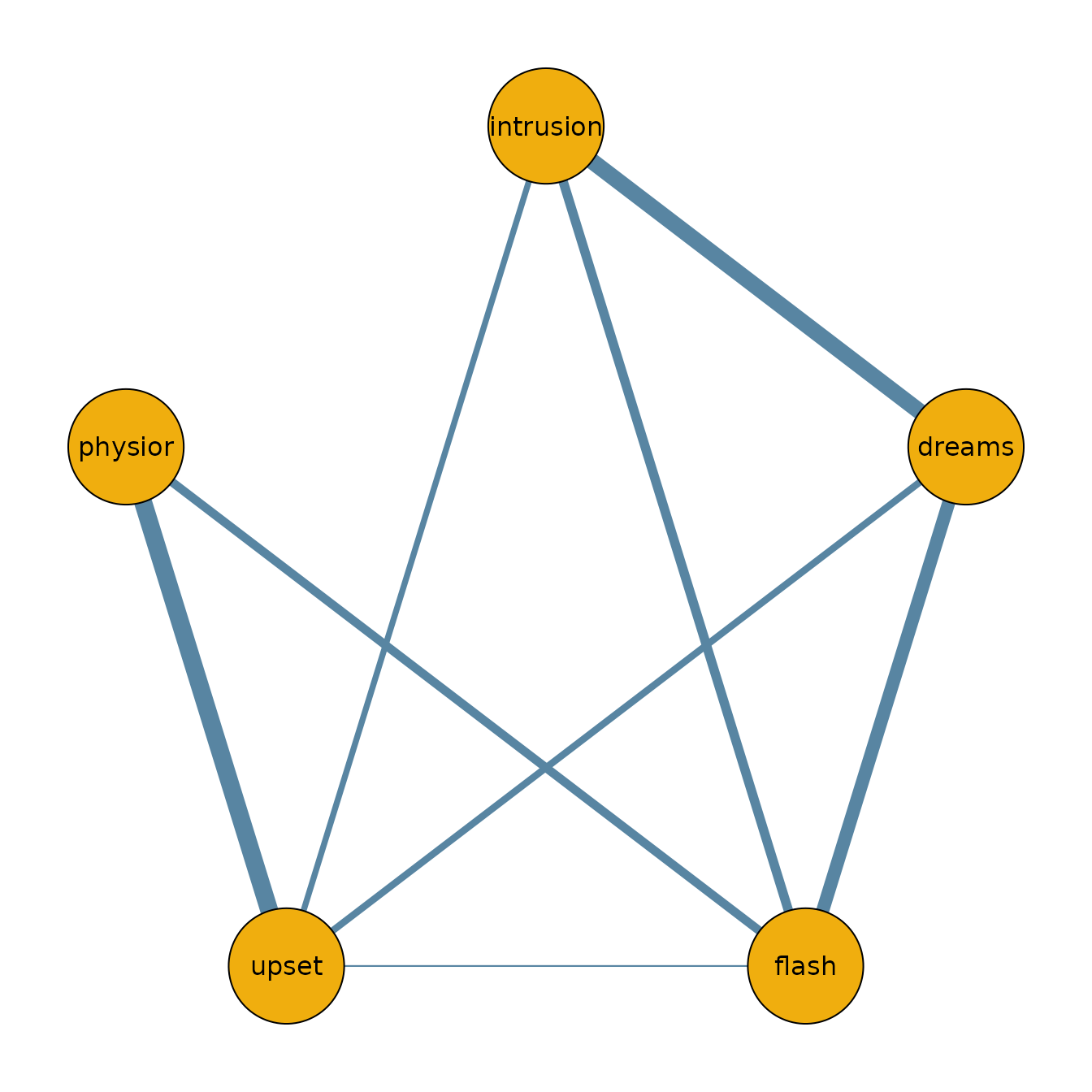
#> physior      0.9315 0.0405 1.0000 1.0000  0.0000

Network plot

To visualize the network structure, we threshold the posterior inclusion probabilities at 0.5 and plot the resulting adjacency matrix.

library(qgraph)

median_probability_network = coef(fit)$pairwise
median_probability_network[coef(fit)$indicator < 0.5] = 0.0

qgraph(median_probability_network,
  theme = "TeamFortress",
  maximum = 1,
  fade = FALSE,
  color = c("#f0ae0e"), vsize = 10, repulsion = .9,
  label.cex = 1, label.scale = "FALSE",
  labels = colnames(data)
)

Continuous data (GGM)

For continuous variables, bgm() fits a Gaussian graphical model when variable_type = "continuous". The workflow is the same:

fit_ggm = bgm(continuous_data, variable_type = "continuous", seed = 1234)
summary(fit_ggm)

The pairwise effects are partial correlations (off-diagonal entries of the standardized precision matrix). Missing values can be imputed during sampling with na_action = "impute".

Next steps

For comparing groups, see ?bgmCompare or the Model Comparison vignette.
For diagnostics and convergence checks, see the Diagnostics vignette.