Check your priors

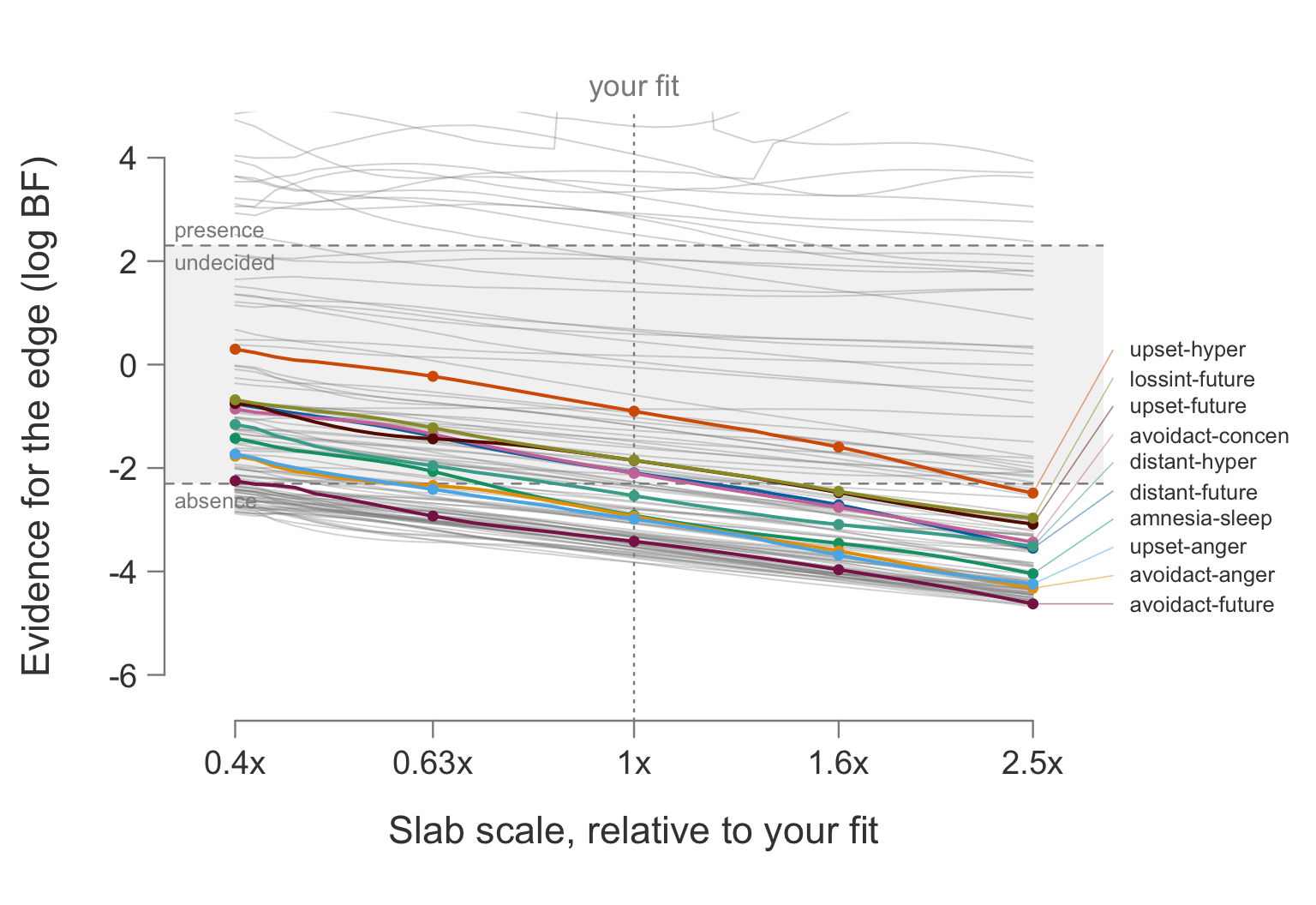
Ninety-one of the 136 edge verdicts of the Wenchuan analysis hold across the whole examined range of prior scales. The colored, named curves are the ten edges whose verdict depends most on that choice, and every verdict that moves anywhere on this plot moves between undecided and a neighboring category.

“Would your conclusions survive a different prior?” is the question every reviewer of a Bayesian analysis is entitled to ask, and for edge verdicts it has real force: the Bayes factor’s evidence of absence is calibrated by how large the weights of a present edge were assumed to be, which is exactly what the interaction prior’s scale says. The honest answer is to redo the analysis under a range of scales and see which verdicts move. Refitting a slow model many times is usually the obstacle; prior_sensitivity_check() gives you the refit-based answer with one call, at well under the cost of one additional fit.

Run it

library(bgms)

fit = bgm(Wenchuan, iter = 1e4, warmup = 5e3, seed = 123)
ps = prior_sensitivity_check(fit, seed = 123)

The check traces every edge’s inclusion Bayes factor as a continuous curve over scales from 0.4 to 2.5 times the one you fitted with. It rests on five anchor fits, and one of them is your original fit, so the verdicts at your own scale are exactly the analysis you already reported; nothing is re-estimated at 1x. The other four anchors are warm-started refits, and one anchor is refit twice so the check knows how much a Bayes factor wobbles between reruns with no prior change at all. On this fit the four refits cost 123 seconds on top of the original fit. That is the whole price of the reviewer’s answer.

Read the report

Printing the result gives the answer first and the machinery last:

ps

Prior sensitivity check: are the edge verdicts robust to the slab scale?
Bayes-factor curve from 0.4x to 2.5x the chosen scale (anchors at 0.4x, 0.63x,
1x, 1.6x, 2.5x; the 1x anchor is the original fit); 136 edges.

91 of 136 verdicts hold across the whole 0.4x-2.5x range; the exceptions are
named below.

  robust (same verdict at every scale)     91
  changed, within run-to-run noise          6
  changed, beyond run-to-run noise         31
  not certifiable (too noisy to assess)     8

31 edges' verdicts genuinely depend on the scale:
  edge               0.4x       0.63x      1x         1.6x       2.5x     
  intrusion-lossint  undecided  absence    absence    absence    absence  
  intrusion-numb     undecided  absence    absence    absence    absence  
  intrusion-sleep    undecided  undecided  undecided  undecided  absence  
  flash-upset        undecided  undecided  absence    absence    absence  
  flash-avoidth      undecided  undecided  undecided  absence    absence  
  flash-sleep        undecided  undecided  absence    absence    absence  
  flash-concen       presence   presence   presence   undecided  undecided
  flash-hyper        undecided  absence    absence    absence    absence  
  upset-distant      undecided  undecided  undecided  undecided  absence  
  upset-numb         undecided  undecided  undecided  absence    absence  
  ...and 21 more; see $edges.

8 edges are too noisy to assess: intrusion-startle, dreams-numb, flash-startle,
upset-avoidact, upset-concen, avoidth-concen, avoidth-hyper, avoidact-startle.
Their Bayes factor sits within Monte Carlo error of an evidence threshold, or
their chains disagree on the verdict, at the chosen scale itself; a rerun with
a fresh seed could flip them without any prior change. Run more iterations to
settle these verdicts before reading their sensitivity.

Verdict counts by scale (at the anchors):
            0.4x 0.63x 1x 1.6x 2.5x
  presence    37    36 35   32   32
  undecided   62    49 39   31   27
  absence     37    51 62   73   77
More absence at wider scales is expected: a wider slab strengthens evidence
against borderline edges.

Note: the chosen scale (1) is much wider than the estimated interactions (about
0.18 [0.148, 0.218]); absence verdicts in particular depend on this choice.

Method:  43-point curve from 5 anchor fits (0.4x to 2.5x the chosen scale),
         joined by importance reweighting; the 1x anchor is the original fit.
         Points with reweighting effective sample size below 400 are not shown.
Refits:  5 nuts refits, warm-started from the original fit, 123 s total.
Noise:   two identical refits at 1.6x differed by up to 0.72 log BF across
         threshold-relevant edges; verdict moves smaller than that are reported
         as run-to-run noise, not prior sensitivity.
         1 edge saturated in one of the two and was left out of that spread.
See ?prior_sensitivity_check for the full construction.

Walk it top to bottom:

The headline. 91 of 136 verdicts hold across the whole range. Within the examined scales, those conclusions belong to the data, not to your prior.
The four categories. Robust edges kept their verdict at every scale. Changed within run-to-run noise (6 edges) moved less than two identical reruns differ from each other, so the check refuses to call that prior sensitivity. Changed beyond run-to-run noise (31 edges) are the genuine movers. Not certifiable (8 edges) are too noisy to assess at all.
The movers table. One row per genuine mover, with its verdict at each anchor scale, so you can see where along the range each verdict changes. Read the direction: a wider slab pulls borderline presence edges into the undecided band and borderline undecided edges into absence. The presence verdicts are the sturdy ones here: of the 35, one (flash-concen) genuinely moves, and then no further than undecided. No edge anywhere crosses between presence and absence.
The not-certifiable list. These eight edges sit within Monte Carlo error of a threshold at the chosen scale itself, or their chains disagree, so a rerun with a fresh seed could flip them without any prior change. They need more iterations, not interpretation.
Verdict counts by scale. The same drift, summarized: absence grows from 37 edges at 0.4x to 77 at 2.5x. The report says why: a wider slab strengthens evidence against borderline edges. That is a property of the Bayes factor, not a defect of the check.
The chosen-scale note. The data prefer a scale of about 0.18 [0.148, 0.218]; the analysis used 1. The interaction weights of these data are small, so the conventional unit scale is a deliberately wide assumption, and the absence verdicts near a threshold should be read with that in mind.
The method block. One honesty acknowledgement suffices here: the curve is carried by real refits, not by reweighting one fit beyond its reach. The construction lives in prior_sensitivity_check() and, in full, in the paper.

Read the curve

The figure at the top of the page is one call:

plot(ps)

Each line is one edge’s log inclusion Bayes factor as a continuous function of the slab scale; the dots mark the five anchor fits, and the 1x anchor is your own analysis. The shaded band is the undecided zone between the evidence thresholds, so the plot reads at a glance: a flat curve is a robust edge, and a verdict changes exactly where a curve crosses into or out of the band. The colored, labeled curves are the ten movers with the largest evidence swings (max_labels sets how many are named); the remaining movers stay grey alongside the robust edges, so the movers table in the report, not the figure, is the complete list. Here the curves drift downward nearly in parallel as the slab widens, which is the mechanism from the report’s count table drawn as geometry.

How to report

Report four items and one figure: how many verdicts hold across the whole range; the named edges whose verdicts genuinely depend on the scale, together with the direction of their change; the scale the data prefer next to the scale you chose; and, for any edge that carries a substantive claim, the range of scales over which its verdict holds. The curve figure belongs in an appendix or supplementary material. In a manuscript this takes two sentences:

A prior sensitivity check (prior_sensitivity_check() in bgms) varied the interaction slab scale from 0.4 to 2.5 times the chosen value; <N> of <M> edge verdicts held across the whole range, and no edge moved between presence and absence. The <K> scale-dependent verdicts all moved between undecided and a neighboring category (<named edges and directions>); the data-preferred scale was <s-hat> [<lo>, <hi>] against the chosen <s>.

How to act

Acting on the result follows the report’s categories.

A robust verdict is reported as is. The check has shown that, within the examined range, the conclusion belongs to the data rather than to the scale.
A not-certifiable edge calls for more iterations, not for interpretation.
A genuine mover is a finding, not a nuisance. Its verdict is a joint product of the data and the chosen scale, and the honest report says so and names the scales on which each reading rests. Three responses are defensible: when substantive grounds single out a narrower range of plausible scales and the verdict holds there, report the verdict with those grounds; when no such grounds exist, treat the mover as undecided in the interpretation, whatever its verdict at your chosen scale, and let its stability range say why; and when the edge matters enough, collect more data: sharper Bayes factors sit further from the thresholds.

One response is not defensible: choosing the scale after seeing which verdict it delivers. The check reports sensitivity; it is not a menu.

One extra caution for evidence of absence, visible in the curve figure: a wider slab mechanically strengthens the evidence against borderline edges. When your chosen scale sits far above the scale the data prefer, as it does here, absence verdicts near the threshold are scale-conditional statements and should be reported as such.

What to report

The count: “<N> of <M> edge verdicts held across slab scales from 0.4 to 2.5 times the chosen value; no edge moved between presence and absence.”
The movers, named, with their direction of change; treat a mover as undecided in the interpretation unless substantive grounds pin down a narrower range of scales on which its verdict holds.
The data-preferred scale next to the chosen one: “<s-hat> [<lo>, <hi>] against the chosen <s>.”
For any edge carrying a substantive claim, the range of scales over which its verdict holds.
Not licensed: rerunning the analysis at whichever scale delivers the verdict you prefer.

Where to next

Prior Basics for what the slab scale does and why it has this leverage on the verdicts.
prior_sensitivity_check() for the arguments, the returned object, and the construction of the curve.
The tutorial manuscript that develops the check and its reading in full is in preparation.
Back in the series: From estimation to evidence, the analysis this check certifies.