Edge clustering

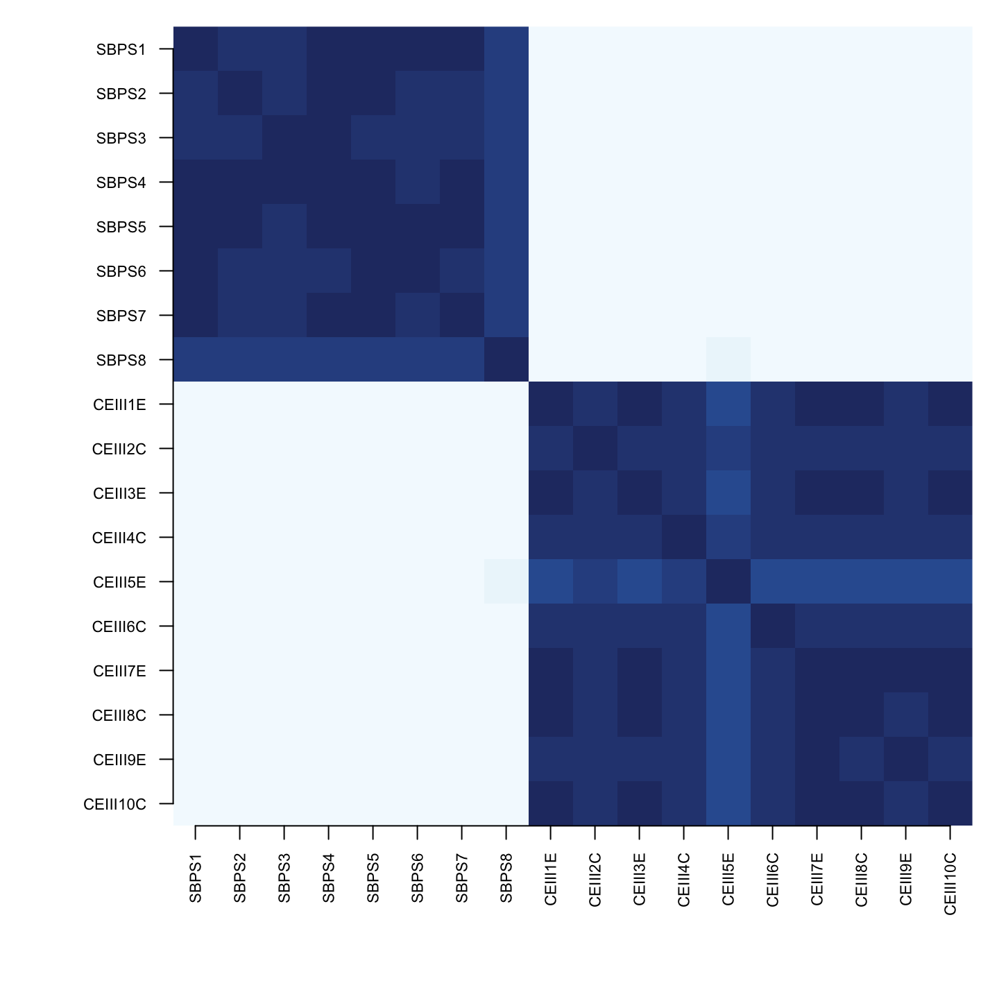
This is the posterior co-clustering matrix of 18 boredom and curiosity items: each cell is the share of posterior draws in which two items landed in the same cluster. Two dark blocks stand out, and they are the two instruments: the eight boredom items of the Short Boredom Proneness Scale cluster together, the ten items of the Curiosity and Exploration Inventory cluster together, and pairs that cross the boundary co-cluster far less often. The model was never told which item belongs to which questionnaire; it recovered the division from the pattern of partial associations, and it reports how sure it is: pairs inside a block co-cluster in 82 to 96 percent of draws, pairs across the boundary in at most 9 percent, and the Bayes factor for clustering over no clustering is about 200.

The usual route to communities is post-hoc: estimate a network, then run a community detection algorithm on the point estimate. That returns a partition, always, with no statement of how sure to be about it, and no way to conclude that there is no community structure. The stochastic block model (SBM) edge prior instead makes the clustering part of the graphical model: cluster assignments, the number of clusters, and the evidence for clustering against no clustering are all estimated together with the network, so every cluster statement arrives with a posterior probability attached (Sekulovski et al., 2025).

The data and the fit

The data come from the French validation of the Short Boredom Proneness Scale (Martarelli et al., 2023): 490 participants, 18 items on 7-point scales, of which 8 measure boredom proneness (SBPS) and 10 measure curiosity and exploration (CEI-II). The two questionnaires give the analysis a natural question: do the items organize into communities, and do the communities follow the instruments? A copy of the dataset is published with this site, so the code below runs as is.

library(bgms)

martarelli = readRDS(url(
  "https://bayesian-graphical-modelling-lab.github.io/bgms/data/martarelli.rds"
))
items = as.data.frame(martarelli[, 3:20])

fit = bgm(items, edge_prior = sbm_prior(), iter = 2e4, warmup = 1e4,
          seed = 123)

The call is bgm() with sbm_prior() at its defaults, including lambda = 1: a prior expectation of two clusters, and prior probability \(\exp(-1) \approx 0.37\) on no clustering at all. The run length is the one deliberate setting, and it earns its place on this page. At the package defaults (2,000 warmup, 2,000 sampling iterations) this fit prints a warmup warning, and the follow-up checks that MCMC Diagnostics prescribes confirm it is real: largest split-\(\hat{R}\) 1.35, smallest effective sample size 44. Worse, the clustering answer is not yet stable at short lengths; an intermediate run at iter = 1e4 put a Bayes factor of only about 6 on clustering where the converged run below puts about 200. At the length shown, the worst split-\(\hat{R}\) is 1.013 and the smallest effective sample size about 350, with the residual wobble confined to a handful of edges that straddle the two blocks. Budget on the order of ten minutes for the run. The guide’s Edge Clustering page carries the model and the hyperparameter guidance, including settings for when clustering is expected and when the goal is to protect against false positive clusters.

Read the clustering

Everything cluster-related lives in one extractor, extract_sbm(). Its first component is the posterior over the number of clusters:

sbm = extract_sbm(fit)
round(head(sbm$posterior_num_blocks, 4), 3)

  probability
1       0.003
2       0.608
3       0.292
4       0.079

The rows are numbers of clusters, and the posterior concentrates on two: probability 0.61 on two clusters, 0.29 on three, and 0.003 on no clustering at all. The Bayes factor tests compare these posterior probabilities with the prior odds implied by the shifted-Poisson prior on the number of clusters; both tests are derived in the guide’s Testing for clustering section.

p = sbm$posterior_num_blocks$probability
names(p) = rownames(sbm$posterior_num_blocks)
round(c(
  # H1: some clustering (B > 1) vs H0: none; prior odds exp(lambda) - 1
  clustering   = ((1 - p["1"]) / p["1"]) / (exp(1) - 1),
  # H1: B = 2 vs H2: B = 1; prior odds 1 at lambda = 1
  two_vs_one   = p["2"] / p["1"],
  # H1: B = 2 vs H2: B = 3; prior odds 2 at lambda = 1
  two_vs_three = (p["2"] / p["3"]) / 2
), 2)

  clustering.1   two_vs_one.2 two_vs_three.2 
        201.96         211.54           1.04

Read the three together. The data support clustering over no clustering (Bayes factor about 200), and two clusters over one (about 212). But two clusters against three is undecided (about 1.04): the data are confident that structure exists and agnostic about whether a third community splits off. That second-order honesty is exactly what the post-hoc route cannot give you; a community detection algorithm handed you one partition and no warning.

The allocations say which items go together:

split(rownames(sbm$posterior_mean_coclustering_matrix),
      sbm$posterior_mode_allocations)

$`1`
[1] "SBPS1" "SBPS2" "SBPS3" "SBPS4" "SBPS5" "SBPS6" "SBPS7" "SBPS8"

$`2`
 [1] "CEIII1E"  "CEIII2C"  "CEIII3E"  "CEIII4C"  "CEIII5E"  "CEIII6C" 
 [7] "CEIII7E"  "CEIII8C"  "CEIII9E"  "CEIII10C"

The modal partition is the two questionnaires, exactly: all eight SBPS items in one cluster, all ten CEI-II items in the other. The co-clustering matrix quantifies how firm each part of that statement is:

cm = sbm$posterior_mean_coclustering_matrix
z = sbm$posterior_mode_allocations
same = outer(z, z, "==")[upper.tri(cm)]
cc = cm[upper.tri(cm)]
round(rbind(within = range(cc[same]), between = range(cc[!same])), 2)

        [,1] [,2]
within  0.82 0.96
between 0.00 0.09

Pairs inside a block co-cluster in 82 to 96 percent of draws; pairs that cross the boundary do so in at most 9. That is what the figure at the top of the page shows; it was drawn from the extractor’s co-clustering matrix directly:

p = nrow(cm)
op = par(mar = c(6.5, 6.5, 1, 1))
image(1:p, 1:p, cm[, p:1], col = hcl.colors(20, "Blues", rev = TRUE),
      axes = FALSE, xlab = "", ylab = "")
axis(1, at = 1:p, labels = rownames(cm), las = 2, cex.axis = 0.7)
axis(2, at = p:1, labels = colnames(cm), las = 1, cex.axis = 0.7)
par(op)

Report the partition and this matrix together: a partition without its co-clustering matrix hides exactly the uncertainty this analysis exists to expose.

The edges still get verdicts

The SBM prior is an edge prior, so the fit is still a full analysis of the network itself, and every tool from the earlier pages applies:

table(verdicts(fit)$verdict)


 presence undecided   absence 
       37        24        92

The edge prior is part of the model, and the inclusion Bayes factors inherit it: under the SBM, an edge between two items that the clustering places together is a priori more plausible than one that crosses the boundary.

What a cluster is not

A cluster here is structure in edge inclusion probabilities under this prior: items in the same block are modeled as more likely to share edges with each other than with the rest. It is not a causal module, not a latent factor, and not proof that the two questionnaires measure distinct constructs; none of those readings are licensed by a partition of a partial association structure. The finding is narrower and still worth having: conditional on everything else, boredom items predict boredom items and curiosity items predict curiosity items far more than they predict each other.

The complement matters too. On data without block structure, this same analysis reports that honestly: the posterior favors a single cluster, the clustering Bayes factor drops below one, and the co-clustering matrix turns diffuse instead of block-diagonal. An uncertain or absent clustering is not a failed analysis; it is a finding, and a caution against over-reading the apparent groupings that any network drawing produces by placing connected nodes near each other.

What to report

The clustering test with the prior it rests on: “The Bayes factor for clustering against no clustering was \(\text{BF} = \texttt{<value>}\) under sbm_prior() with \(\lambda = \texttt{<value>}\),” and its verdict: support, evidence against, or undecided.
The posterior over the number of clusters, the modal allocations, and the co-clustering matrix (or its within- and between-block ranges) as the uncertainty statement for the partition.
The hyperparameters, if changed from the defaults: they encode how strongly the prior expects clustering.
Not licensed: reading groups in a network drawing as clusters, reporting a partition without its allocation uncertainty, treating a cluster as a latent variable, or reading a Bayes factor near one as evidence that there are no clusters.

Where to next

Edge Clustering for the model: the block structure on inclusion probabilities, the two Bayes factor tests, and hyperparameter guidance.
sbm_prior() and extract_sbm() for the arguments and the return value.
Sekulovski et al. (2025) for the step-by-step tutorial behind this analysis, and Martarelli et al. (2023) for the study the data come from.
Back in the series: From estimation to evidence, the single-network analysis this page builds on.

References

Martarelli, C. S., Baillifard, A., & Audrin, C. (2023). A trait-based network perspective on the validation of the French Short Boredom Proneness Scale. European Journal of Psychological Assessment, 39(6), 390–399. https://doi.org/10.1027/1015-5759/a000718

Sekulovski, N., Arena, G., Haslbeck, J. M. B., Huth, K. B. S., Friel, N., & Marsman, M. (2025). A stochastic block prior for clustering in graphical models. Manuscript Submitted for Publication. https://osf.io/preprints/psyarxiv/29p3m_v3