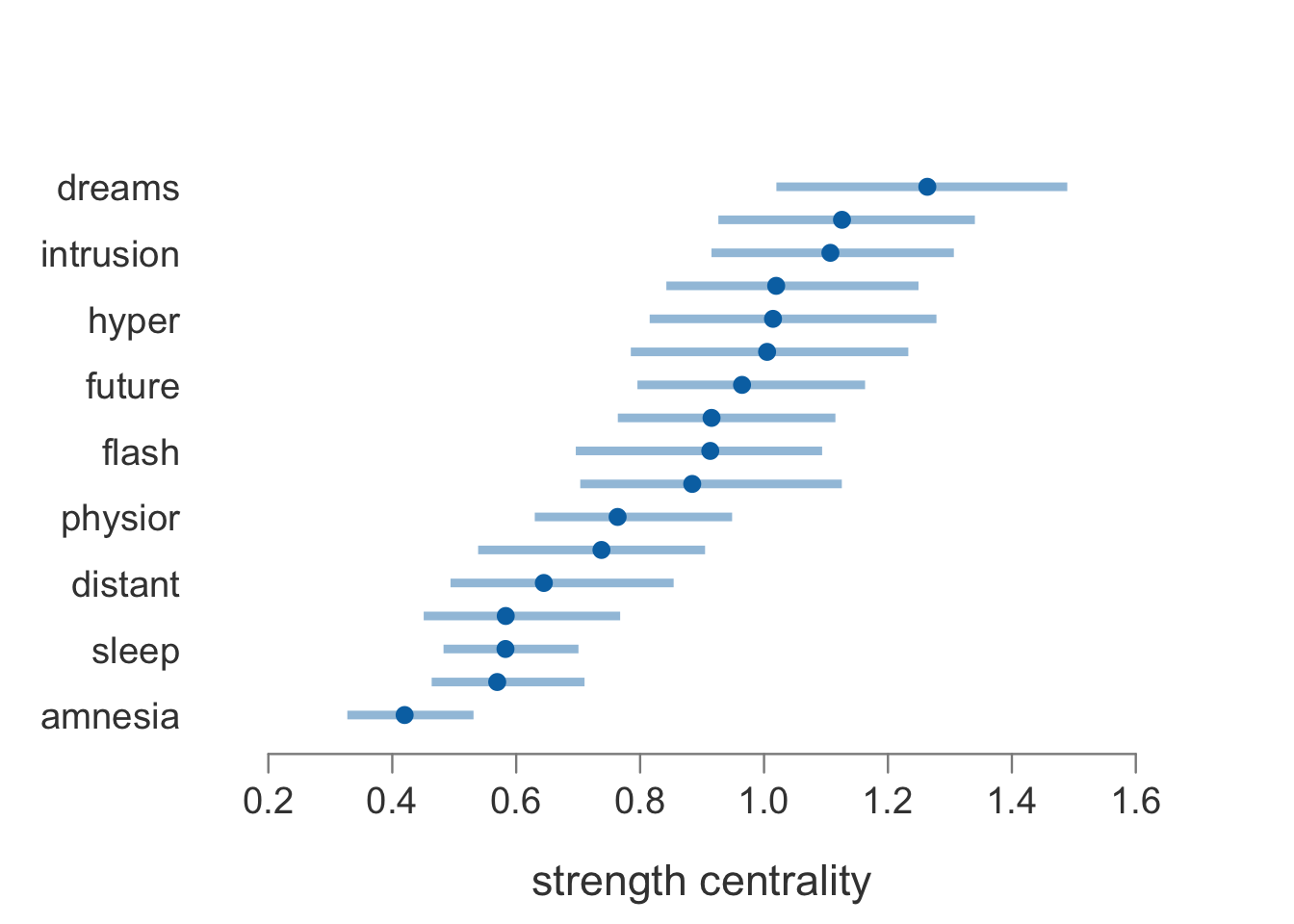
Functions to extract specific components from fitted bgms and bgmCompare objects. Executed examples on this page use a bgm() fit of the Wenchuan data (fit = bgm(Wenchuan, iter = 1e4, warmup = 5e3, seed = 123)).
Unless noted otherwise, extractor functions use one argument:
bgms_object: a fitted bgms or bgmCompare object.
extract_arguments
Retrieve the arguments used when fitting a model with bgm() or bgmCompare().
extract_arguments(bgms_object)
Returns a named list containing all arguments passed to the fitting function, including data dimensions, prior settings, and MCMC configuration.
extract_main_effects
Retrieve posterior mean main-effect parameters.
extract_main_effects(bgms_object)
The structure depends on the model type:
GGM (bgms): NULL. GGM models have no main effects.
OMRF (bgms): A numeric matrix (p x max_categories) of posterior mean category thresholds. Columns beyond the number of categories for a variable are NA.
Mixed MRF (bgms): A list with $discrete (threshold matrix) and $continuous (means matrix).
bgmCompare: A matrix with one row per post-warmup iteration, containing posterior samples of baseline main-effect parameters.
extract_pairwise_interactions
Retrieve posterior samples of partial association parameters.
extract_pairwise_interactions(bgms_object)
Returns a matrix with one row per post-warmup iteration and one column per edge. For bgmCompare, columns correspond to baseline partial association parameters.
extract_centrality
Evaluate a node centrality on every posterior draw of the network, giving the posterior distribution of each node’s centrality.
extract_centrality(bgms_object, measure ="strength", group =1, ...)
Argument
Description
bgms_object
A fitted bgms or bgmCompare object.
measure
Character; the centrality to evaluate. Currently "strength" (default) is the only accepted value, the sum of the absolute weights of a node’s edges. Anything else is an error.
group
For a bgmCompare fit: a single group index, giving that group’s centrality, or two indices, giving the difference in centrality between them (the first minus the second). Default: 1. Ignored for a bgms fit, which has one network.
...
Passed to methods.
Returns a numeric matrix of class "bgms_centrality" with one row per posterior draw and one column per variable, carrying measure as an attribute.
summary() returns a data frame with one row per variable, ordered by decreasing posterior mean: node, mean, lower, upper, and p_most_central, the posterior probability that the node has the largest centrality of all nodes. For a difference between two groups the last column is p_positive instead, the posterior probability that the node’s centrality is higher in the first group than in the second; which node is most central is not a question a difference answers. plot() draws each node’s posterior mean with its credible interval, nodes ordered by mean, and returns x invisibly.
Details
The centrality is evaluated on the model-averaged pairwise draws, in which an edge excluded at a given iteration contributes exactly zero. Structural uncertainty therefore propagates into the centrality without any extra step: a node whose edges are themselves uncertain gets a wide centrality posterior, which is the honest summary. Conditioning on the included-only draws instead would report each node’s centrality in the models where its edges happen to be present, which is a different and generally larger quantity.
Strength sums absolute edge weights, so positive and negative associations both add to a node’s total involvement rather than cancelling.
For a bgmCompare() fit each group’s network is rebuilt on every draw as baseline + (P %*% differences), with the fit’s own contrast projection P, rather than from posterior means. That is what carries the uncertainty through: with group = c(1, 2) the credible interval is the interval of the difference in a node’s centrality, which answers whether the groups differ in it directly, where two separately drawn intervals do not.
Read a centrality difference with care, and as numbers rather than as a picture; plot() declines to draw one. Strength sums absolute weights, so a difference of zero can mean identical networks or compensating edge differences, and its sign says nothing about which edges moved. verdicts() is the per-difference evidence.
A difference also has a point mass at exactly zero, from the draws in which every one of the node’s difference indicators is excluded and the two groups share the network. p_positive and its mirror therefore need not sum to one, and a node can have a positive posterior mean with p_positive well below 0.5: the remaining mass is on no difference at all, which is the model averaging reporting itself.
Two estimators of the same quantity are available. The default "rb" (Rao-Blackwellized) averages the one-step inclusion draw \(J_t = \gamma_t + (1 - 2\gamma_t)\,\alpha_t\) recorded at each birth/death proposal, where \(\gamma_t\) is the indicator state before the move and \(\alpha_t\) the proposal’s acceptance probability; "raw" averages the binary indicator draws themselves. The RB average has lower variance and, in exact arithmetic, always lies strictly inside \((0, 1)\) — though for edges with overwhelming per-iteration evidence it still rounds to exactly 0 or 1 in double precision. It changes only the summary, not the sampler: it inherits the chain’s mixing and does not rescue a chain that failed to explore the model space.
Returns a symmetric p x p matrix of posterior inclusion probabilities:
Here the intrusion–dreams edge saturates at probability 1, while intrusion–upset sits around 0.66 — the data do not clearly decide that edge. See Edge Selection for turning these into Bayes factors, and extract_inclusion_bf() for a Bayes-factor estimator that stays finite for saturated edges up to the numerical bound described there. - bgmCompare: Diagonal entries are main-effect inclusion probabilities; off-diagonal entries are pairwise difference inclusion probabilities. Requires difference_selection = TRUE. With estimator = "rb", indicators that were not selected (e.g. main-effect differences when main_difference_selection = FALSE) are returned as NA.
extract_inclusion_bf
Compute inclusion Bayes factors from the Rao-Blackwellized odds accumulators recorded during sampling.
extract_inclusion_bf( bgms_object,log =FALSE)
log selects the scale of the return. The default FALSE gives the inclusion Bayes factor itself; TRUE gives its natural logarithm.
For each indicator, the sampler accumulates the birth/death acceptance probabilities on the acceptance-probability scale, so the posterior inclusion odds follow from the exact identity
where \(n_{01}\) and \(n_{10}\) sum the acceptance probabilities of birth and death proposals and \(n_0\), \(n_1\) count them. Because \(1 - \alpha\) is never formed per draw, the odds stay finite down to log acceptance probabilities of about \(-745\): edges whose inclusion-probability average rounds to 0 or 1 still receive a finite Bayes factor here.
The prior inclusion odds are divided out edge by edge, so the returned value is the inclusion Bayes factor rather than the posterior odds (the two coincide only at a prior inclusion probability of \(\tfrac{1}{2}\)). For bgm() fits the prior odds come from extract_prior_inclusion_probabilities(); for continuous or stochastic-block models that call may run and cache a short prior-only chain. For bgmCompare() fits the exchangeable difference prior supplies a single prior inclusion probability; a stochastic-block difference prior has no single marginal, so the result is left as posterior odds there.
Returns a symmetric p x p matrix of inclusion Bayes factors, or of their natural logarithms when log = TRUE. Entries are NA for indicators that were never updated and +Inf when no exclusion evidence remains. An entry with no inclusion evidence left is -Inf on the log scale and 0 on the Bayes factor scale. For bgms the diagonal is NA; for bgmCompare the diagonal holds main-effect difference Bayes factors.
          intrusion    dreams    flash  upset
intrusion        NA 2.12e+119 1.82e+05 1.9800
dreams    2.12e+119        NA 1.04e+32 7.8400
flash      1.82e+05  1.04e+32       NA 0.0737
upset      1.98e+00  7.84e+00 7.37e-02     NA
The intrusion–dreams edge, whose inclusion probability saturates at 1 above, here receives a Bayes factor of about \(2 \times 10^{119}\): astronomically strong evidence, but quantified rather than Inf.
The accumulators are exact on the log scale everywhere, while the Bayes factor scale saturates at double precision: an entry whose log exceeds about 709.78 nats (a Bayes factor beyond about \(1.8 \times 10^{308}\)) comes back as +Inf under the default even though its log-scale value is finite. Use log = TRUE when you need to separate such extreme evidence:
          intrusion dreams flash upset
intrusion        NA 274.76 12.11  0.68
dreams       274.76     NA 73.72  2.06
flash         12.11  73.72    NA -2.61
upset          0.68   2.06 -2.61    NA
extract_prior_inclusion_probabilities
Compute prior inclusion probabilities, in the same shape and orientation as extract_posterior_inclusion_probabilities(), so the two can be combined element-wise into prior and posterior inclusion odds — and from there into inclusion Bayes factors.
bgms_object must be a fitted bgms object with edge_selection = TRUE. Returns a symmetric matrix of prior inclusion probabilities with the variable names as row and column names and a zero diagonal.
For models without a continuous block of at least two variables (ordinal MRFs, mixed models with a single continuous variable), the prior inclusion probability is simply the edge prior’s marginal: the fixed probability for bernoulli_prior(), \(\alpha / (\alpha + \beta)\) for beta_bernoulli_prior(), and the mixture of the within- and between-block means for sbm_prior().
Under the default precision_graph_prior = "hierarchical" in bgm() the same holds for a continuous block: \(p(K \mid \Gamma)\) is normalized per graph, so integrating \(K\) out returns the edge prior exactly and every edge class keeps the edge-prior marginal. Nothing is read off a table or estimated by a chain, and the function returns quickly.
Under precision_graph_prior = "joint" the graph marginal is instead reweighted by a per-graph normalizing constant, so the prior inclusion probability of a continuous-continuous edge differs from the edge-prior marginal — even at delta = 0. This function then returns the actual reweighted probabilities: for bernoulli_prior() and beta_bernoulli_prior() they are read from the same cached normalizing-constant table that corrects the fit’s hyperparameter updates; for sbm_prior() (and slab families without a table) they are estimated by a prior-only chain run with the fit’s own prior settings, controlled by iter and warmup. That estimate is cached on the fit, and recompute = TRUE re-runs it. Building an uncached table takes minutes; the build is announced and draws a progress bar rather than pausing silently.
In mixed models only continuous-continuous edges live in the joint block, so on a joint fit the matrix carries up to three distinct values: discrete-discrete, continuous-continuous, and cross edges.
extract_indicator_priors
Retrieve the prior specification used for inclusion indicators.
extract_indicator_priors(bgms_object)
Returns a named list describing the prior structure, including the prior type and hyperparameters:
bgms: Requires edge_selection = TRUE. Returns the prior type ("Bernoulli", "Beta-Bernoulli", or "Stochastic-Block") and associated hyperparameters.
bgmCompare: Requires difference_selection = TRUE. Returns the difference prior specification.
extract_group_params
Compute group-specific parameter estimates by combining baseline parameters and group differences.
extract_group_params(bgms_object)
bgms_object must be a fitted bgmCompare object.
Returns a list with main_effects_groups (main effects per group) and pairwise_effects_groups (pairwise effects per group).
extract_sbm
Retrieve posterior summaries from a model fitted with the Stochastic Block prior.
extract_sbm(bgms_object)
Works on both bgms and bgmCompare fits.
For bgms: requires edge_selection = TRUE and edge_prior = sbm_prior(...).
For bgmCompare: requires difference_selection = TRUE and difference_prior = sbm_prior(...). The clustering applies to the off-diagonal (pairwise) difference inclusions.
Returns a list with:
posterior_num_blocks — Posterior probabilities for each possible number of clusters, computed under the shifted-Poisson prior on the number of clusters (see Edge Clustering).
posterior_mean_allocations — Posterior mean cluster allocations.
Returns a named list with ESS values for each parameter type present in the model (e.g., main, pairwise, indicator). ESS values match coda::effectiveSize. For implementation details, see the Technical Manual.
Two elements are composite rather than raw-chain quantities. The indicator element is the n_eff column of summary(fit)$indicator: the ESS of the Rao-Blackwellized inclusion draws, and therefore the ESS of the inclusion probability the fit reports. It is read from the same continuous chain that extract_rhat() uses for indicators, and it measures precision conditional on exploration. Read it beside the directional transition counts n0->1 and n1->0, which carry the exploration itself; see MCMC Diagnostics.
estimator has one live value, "rb". The alternative, estimator = "mixt" — the transition-based ESS of the binary indicator chain — is deprecated as of 0.2.0.0: the simple two-state process it assumes describes many edge chains poorly, so the statistic no longer feeds any inclusion verdict. Passing it warns and still returns the statistic. n_eff_mixt is no longer a column of summary(fit)$indicator.
The indicator element is NA wherever the inclusion probability is pinned at its bound and no precision is left to estimate; see extract_rhat() for the exact rule. Fits made with bgms < 0.2.0.0 carry no Rao-Blackwellized draws, so an explicit estimator = "rb" errors there.
The pairwise element is the composite ESS of the model-averaged edge weight, which combines inclusion and slab uncertainty.
Low values relative to the total number of retained draws signal slow mixing for that parameter; see MCMC Diagnostics for guidance.
extract_rhat
Retrieve R-hat convergence diagnostics for all parameters.
extract_rhat(bgms_object)
Returns a named list with R-hat values for each parameter type present in the model (e.g., main, pairwise, indicator). The statistic is split-R-hat (Vehtari et al., 2021): each chain is split in half and the Gelman-Rubin formula is applied to the half-chains, so that within-chain drift is detected as well as between-chain disagreement. No degrees-of-freedom adjustment is applied. For implementation details, see diagnostics in the Technical Manual.
The indicator element is computed on the continuous Rao-Blackwellized inclusion draws. It is NA where those draws are exactly constant, with the inclusion probability pinned at its bound. Draws that vary too little for the autocorrelation machinery, without being exactly constant, keep a finite Rhat while mcse and n_eff are NA. Neither set is the same as the set of edges whose binary indicator never flipped.
NoteOne failure mode these diagnostics do not see
Chains can agree that an edge is included while disagreeing about the magnitude of its weight — for instance when the weight’s posterior has more than one mode and different chains settle in different ones. The indicator diagnostics cannot see this by construction, and the pooled-draw pairwise R-hat responds only weakly when inclusion is intermittent, because the zeros the excluded draws contribute dominate the between-chain comparison.
When it matters, compare each edge’s weight across chains using only the draws in which that edge is included, reading the per-chain pairwise and indicator draws out of fit$raw_samples. A dedicated diagnostic for this is planned for a future release.
extract_precision
Retrieve the posterior mean precision matrix.
extract_precision(bgms_object)
bgms_object must be a fitted bgms object (GGM or mixed MRF).
Returns a symmetric p x p matrix (or the continuous block submatrix for mixed MRFs) containing the posterior mean precision matrix \(\boldsymbol{\Theta}\).
extract_partial_correlations
Retrieve the posterior mean partial correlation matrix.
extract_partial_correlations(bgms_object)
bgms_object must be a fitted bgms object (GGM or mixed MRF).
Returns a symmetric matrix of partial correlations, computed by standardizing the precision matrix: \(\rho_{ij} = -\Theta_{ij} / \sqrt{\Theta_{ii}
\Theta_{jj}}\).
extract_log_odds
Retrieve the posterior mean log-odds matrix.
extract_log_odds(bgms_object)
bgms_object must be a fitted bgms object (OMRF or mixed MRF).
Returns a symmetric matrix of log adjacent-category odds ratios. For the ordinal MRF, \(\text{log-odds}_{ij} = 2 \omega_{ij}\).
Deprecated functions
extract_category_thresholds() — Renamed to extract_main_effects().
extract_edge_indicators() — Renamed to extract_indicators().
extract_pairwise_thresholds() — Renamed to extract_main_effects().
Vehtari, A., Gelman, A., Simpson, D., Carpenter, B., & Bürkner, P.-C. (2021). Rank-normalization, folding, and localization: An improved \(\widehat{R}\) for assessing convergence of MCMC (with discussion). Bayesian Analysis, 16(2), 667–718. https://doi.org/10.1214/20-BA1221