Getting Started

bgms implements Bayesian estimation and edge selection for graphical models of mixed binary, ordinal, and continuous variables. Networks are estimated at the level of conditional associations: an edge between two variables indicates a direct relationship that persists after accounting for all other variables in the model.

The package has two main entry points:

For background on graphical models and the Bayesian approach, see Graphical Models and The Bayesian Approach.

Installation

From CRAN

install.packages("bgms")

Development version

if(!requireNamespace("remotes")) {
  install.packages("remotes")
}
remotes::install_github("Bayesian-Graphical-Modelling-Lab/bgms@develop")

The @develop suffix matters. Without it install_github() takes the default branch, which carries the released CRAN lineage rather than the development version.

Fitting a model

The main function is bgm(). It accepts a data frame or matrix of mixed binary, ordinal, and continuous variables and estimates a Markov random field.

The Wenchuan dataset is included in the package, and contains ordinal measures of symptoms of posttraumatic stress from 362 survivors of the 2008 Wenchuan earthquake.

library(bgms)

data(Wenchuan)
head(Wenchuan)
     intrusion dreams flash upset physior avoidth avoidact amnesia lossint
[1,]         2      2     2     2       3       2        3       2       3
[2,]         2      2     2     3       3       3        3       2       3
[3,]         2      4     4     4       3       3        3       5       4
[4,]         2      1     2     2       1       1        2       2       2
[5,]         2      2     2     2       2       2        2       2       3
[6,]         4      3     2     2       2       2        3       3       2
     distant numb future sleep anger concen hyper startle
[1,]       2    2      1     3     4      3     4       2
[2,]       3    2      2     3     3      2     3       3
[3,]       3    2      3     4     4      4     3       4
[4,]       1    1      2     2     1      2     3       3
[5,]       2    2      2     3     2      3     2       3
[6,]       2    2      3     2     3      2     3       2

For illustration, we select five symptoms from the Wenchuan dataset — intrusive memories, disturbing dreams, flashbacks, emotional upset, and physical reactions — so that the output fits on screen:

fit = bgm(Wenchuan[, 1:5], seed = 1234)

By default, bgm() runs four parallel MCMC chains using the No-U-Turn Sampler (NUTS) — the default sampling algorithm — in combination with Bayesian edge selection. Here we use seed = 1234 for reproducibility. If the sampler diagnostics indicate persistent problems, refit with update_method = "adaptive-metropolis".

Posterior summaries

summary(fit)
Posterior summaries from Bayesian estimation:

Category thresholds: 
                mean  mcse    sd    n_eff  Rhat
intrusion (2)  0.476 0.003 0.232 5873.432 1.001
intrusion (3) -1.908 0.006 0.338 3201.453 1.002
intrusion (4) -4.856 0.010 0.548 2820.656 1.002
intrusion (5) -9.534 0.016 0.881 2988.276 1.002
dreams (2)    -0.594 0.002 0.191 6193.119 1.001
dreams (3)    -3.790 0.005 0.337 4973.439 1.002
... (use `summary(fit)$main` to see full output)

Pairwise interactions:
                   mean  mcse    sd    n_eff share_incl  Rhat
intrusion-dreams  0.315 0.000 0.033 7784.844      0.000 1.000
intrusion-flash   0.169 0.000 0.031 7893.727      0.000 1.000
intrusion-upset   0.097 0.001 0.035  947.703      0.873 1.002
intrusion-physior 0.100 0.001 0.033 1402.358      0.793 1.002
dreams-flash      0.250 0.000 0.030 9592.002      0.000 1.000
dreams-upset      0.114 0.000 0.028 3988.563      0.121 1.001
... (use `summary(fit)$pairwise` to see full output)

Inclusion probabilities:
                   mean  mcse    sd    n_eff  Rhat n0->1 n1->0
intrusion-dreams  1.000       0.000                    0     0
intrusion-flash   1.000       0.000              1     0     0
intrusion-upset   0.954 0.011 0.205  379.316 1.007    23    23
intrusion-physior 0.970 0.008 0.165  466.518 1.013    19    19
dreams-flash      1.000       0.000                    0     0
dreams-upset      0.995 0.001 0.067 2486.973 1.005     4     4
... (use `summary(fit)$indicator` to see full output)
Note: NA values are suppressed in the print table; they occur for indicators
that were not updated or whose draws are constant, so ESS/Rhat are undefined.
`summary(fit)$indicator` still contains all computed values.

Use `summary(fit)$<component>` to access full results.
Use `extract_log_odds(fit)` for log odds ratios.
See the `easybgm` package for other summary and plotting tools.

The summary shows posterior means, standard deviations, Monte Carlo standard errors (MCSE), effective sample sizes (ESS), and R-hat values for each parameter. For partial associations, it also reports posterior inclusion probabilities because we used edge selection. For a full description of the output structure, see Model Output; for guidance on interpreting the convergence diagnostics (ESS and R-hat), see MCMC Diagnostics.

Posterior means

coef(fit)
$main
             cat (1)   cat (2)   cat (3)    cat (4)
intrusion  0.4759198 -1.908039 -4.855923  -9.533872
dreams    -0.5940868 -3.790280 -7.120179 -11.553219
flash     -0.1032762 -2.564714 -5.368187  -9.675458
upset      0.4192317 -1.308041 -3.380035  -7.047338
physior   -0.6163672 -3.174850 -6.231561 -10.582211

$pairwise
           intrusion      dreams       flash       upset     physior
intrusion 0.00000000 0.315402244 0.168831614 0.097379159 0.099761224
dreams    0.31540224 0.000000000 0.249762223 0.113622854 0.003511578
flash     0.16883161 0.249762223 0.000000000 0.004631963 0.152974419
upset     0.09737916 0.113622854 0.004631963 0.000000000 0.354885509
physior   0.09976122 0.003511578 0.152974419 0.354885509 0.000000000

$indicator
          intrusion     dreams      flash      upset    physior
intrusion 0.0000000 1.00000000 1.00000000 0.95420066 0.97042544
dreams    1.0000000 0.00000000 1.00000000 0.99514226 0.07790594
flash     1.0000000 1.00000000 0.00000000 0.09621877 1.00000000
upset     0.9542007 0.99514226 0.09621877 0.00000000 1.00000000
physior   0.9704254 0.07790594 1.00000000 1.00000000 0.00000000

coef() returns posterior mean matrices: $pairwise contains the partial associations and $indicator contains edge inclusion probabilities.

The network, split by evidence

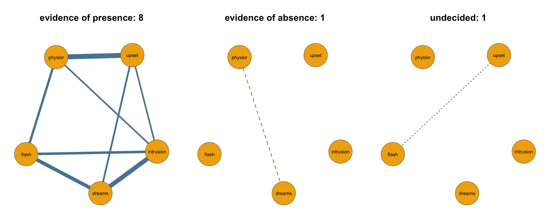
A single network drawing has to make every pair either an edge or a blank, and a blank cannot say whether the data ruled the pair out or simply had too little to say about it. Because bgms returns an inclusion Bayes factor for every pair, you do not have to make that choice. The network is drawn as three panels on one shared layout: the pairs the data support, the pairs the data rule out, and the pairs the data cannot decide. This is the edge evidence plot, and it is the display this documentation uses for every network result.

The categories come from extract_inclusion_bf() at an inclusion Bayes factor of 10 in either direction. See Edge Selection for why the Bayes factor, and not the inclusion probability on its own, is what licenses a claim about an edge. plot(fit) draws a rudimentary version of this display in one call, and the easybgm package offers more elaborate plotting and summary functions on top of bgms. The drawing below uses the qgraph package directly (Epskamp et al., 2012), with every styling choice under your control.

library(qgraph)

plot_edge_evidence = function(fit, labels, node_color, threshold = 10,
                              seed = 1234) {
  bf = extract_inclusion_bf(fit)
  weights = coef(fit)$pairwise

  presence = bf >= threshold
  absence = bf <= 1 / threshold
  undecided = !presence & !absence
  diag(presence) = diag(absence) = diag(undecided) = FALSE

  # One layout, computed from every pair, so the three panels match node
  # for node.
  set.seed(seed)
  shared = qgraph(abs(weights), layout = "spring", repulsion = 0.9,
                  DoNotPlot = TRUE)$layout

  panel = function(edges, label, count, ...) {
    qgraph(edges, layout = shared, labels = labels, fade = FALSE,
           color = node_color, vsize = 17, label.scale.equal = TRUE,
           border.color = "grey30", mar = c(3, 4, 8, 4), ...)
    mtext(sprintf("%s: %d", label, count), side = 3, line = 1.2,
          cex = 0.95, font = 2)
  }

  par(mfrow = c(1, 3))
  panel(weights * presence, "evidence of presence", sum(presence) / 2,
        theme = "TeamFortress", edge.width = 1.1)
  panel(absence * 1, "evidence of absence", sum(absence) / 2,
        edge.color = "#A66A1E", lty = 2, edge.width = 1.1)
  panel(undecided * 1, "undecided", sum(undecided) / 2,
        edge.color = "#8A8578", lty = 3, edge.width = 1.4)
}

plot_edge_evidence(fit, colnames(Wenchuan)[1:5], "#f0ae0e")

Each panel licenses a different statement.

  • Evidence of presence. For these eight pairs the data favor a direct association, one that survives conditioning on the other three symptoms. Only this panel is weighted: line width is the posterior mean partial association, so the effect sizes live here.
  • Evidence of absence. dreams-physior is the one pair the data actively rule out, with an inclusion Bayes factor of about 0.08, or roughly 12 to 1 against. That is a positive statement of conditional independence, and it is the statement an estimation workflow cannot make: there, a missing edge might just as well mean too little data. The panel is drawn dashed and at uniform width because for these pairs the classification, not a weight, is the result.
  • Undecided. flash-upset is the pair these data have too little to say about. Its Bayes factor of about 0.11 sits just inside the undecided band, so it is neither supported nor ruled out.

This is why the site does not draw the bare thresholded network. Keeping only the edges with posterior inclusion probability of 0.5 or more, the median probability model, would reproduce exactly the eight edges of the first panel and leave dreams-physior and flash-upset equally blank. One of those two blanks is a finding; the other is an open question, and the drawing would not tell you which is which.

Continuous data

For continuous variables, bgms fits a Gaussian graphical model. The interface is identical; only the variable_type argument changes. (All-continuous data also admit a dedicated Gibbs sampler via update_method = "gibbs", which draws from exact conditionals with nothing to tune — see Gaussian Graphical Model.)

As a continuous-data example, we use the classic examination marks dataset from Mardia et al. (1979). The data contain scores of 88 students on five examinations:

marks = data.frame(
  mechanics  = c(77,63,75,55,63,53,51,59,62,64,52,55,50,65,31,60,44,42,62,31,
                 44,49,12,49,54,54,44,18,46,32,30,46,40,31,36,56,46,45,42,40,
                 23,48,41,46,46,40,49,22,35,48,31,17,49,59,37,40,35,38,43,39,
                 62,48,34,18,35,59,41,31,17,34,46,10,46,30,13,49,18,8,23,30,
                 3,7,15,15,5,12,5,0),
  vectors    = c(82,78,73,72,63,61,67,70,60,72,64,67,50,63,55,64,69,69,46,49,
                 61,41,58,53,49,53,56,44,52,45,69,49,27,42,59,40,56,42,60,63,
                 55,48,63,52,61,57,49,58,60,56,57,53,57,50,56,43,35,44,43,46,
                 44,38,42,51,36,53,41,52,51,30,40,46,37,34,51,50,32,42,38,24,
                 9,51,40,38,30,30,26,40),
  algebra    = c(67,80,71,63,65,72,65,68,58,60,60,59,64,58,60,56,53,61,61,62,
                 52,61,61,49,56,46,55,50,65,49,50,53,54,48,51,56,57,55,54,53,
                 59,49,49,53,46,51,45,53,47,49,50,57,47,47,49,48,41,54,38,46,
                 36,41,50,40,46,37,43,37,52,50,47,36,45,43,50,38,31,48,36,43,
                 51,43,43,39,44,32,15,21),
  analysis   = c(67,70,66,70,70,64,65,62,62,62,63,62,55,56,57,54,53,55,57,63,
                 62,49,63,62,47,59,61,57,50,57,52,59,61,54,45,54,49,56,49,54,
                 53,51,46,41,38,52,48,56,54,42,54,43,39,15,28,21,51,47,34,32,
                 22,44,47,56,48,22,30,27,35,47,29,47,15,46,25,23,45,26,48,33,
                 47,17,23,28,36,35,20,9),
  statistics = c(81,81,81,68,63,73,68,56,70,45,54,44,63,37,73,40,53,45,45,62,
                 46,64,67,47,53,44,36,81,35,64,45,37,61,68,51,35,32,40,33,25,
                 44,37,34,40,41,31,39,41,33,32,34,51,26,46,45,61,50,24,49,43,
                 42,33,29,30,29,19,33,40,31,36,17,39,30,18,31,9,40,40,15,25,
                 40,22,18,17,18,21,20,14)
)
head(marks)
  mechanics vectors algebra analysis statistics
1        77      82      67       67         81
2        63      78      80       70         81
3        75      73      71       66         81
4        55      72      63       70         68
5        63      63      65       70         63
6        53      61      72       64         73
fit_ggm = bgm(marks, variable_type = "continuous", seed = 1234)
summary(fit_ggm)
summary(fit_ggm)
Posterior summaries from Bayesian estimation:

Residual variances:
                                  mean  mcse     sd    n_eff  Rhat
mechanics (residual variance)  206.259 0.385 32.271 7029.464 1.000
vectors (residual variance)     94.168 1.097 17.727  261.245 1.009
algebra (residual variance)     29.950 0.153  4.102  716.650 1.006
analysis (residual variance)   105.775 0.166 16.007 9249.091 1.000
statistics (residual variance) 161.079 0.247 24.178 9573.656 1.000

Pairwise interactions:
                      mean mcse    sd     n_eff share_incl  Rhat
mechanics-vectors    0.001    0 0.001   114.566      0.998 1.024
mechanics-algebra    0.001    0 0.001   116.783      0.997 1.025
mechanics-analysis   0.000    0 0.000 15329.282      0.175 1.000
mechanics-statistics 0.000    0 0.000 24810.749      0.058 1.000
vectors-algebra      0.004    0 0.001  7966.365      0.196 1.000
vectors-analysis     0.000    0 0.000 61928.276      0.484 1.000
... (use `summary(fit)$pairwise` to see full output)

Inclusion probabilities:
                      mean  mcse    sd    n_eff  Rhat n0->1 n1->0
mechanics-vectors    0.502 0.049 0.493   99.487 1.026    82    80
mechanics-algebra    0.552 0.049 0.490  100.501 1.026    90    92
mechanics-analysis   0.002 0.000 0.015 6805.609 1.000    15    15
mechanics-statistics 0.001 0.000 0.008 7209.202 1.002    14    14
vectors-algebra      0.997 0.001 0.055 2646.821 1.003     3     3
vectors-analysis     0.001 0.000 0.010 6248.296 1.000    13    13
... (use `summary(fit)$indicator` to see full output)

Use `summary(fit)$<component>` to access full results.
Use `extract_partial_correlations(fit)` for partial correlations,
and `extract_precision(fit)` for the precision matrix.
See the `easybgm` package for other summary and plotting tools.

The GGM network, split by evidence

The same three panels, the same rule, the same function:

plot_edge_evidence(fit_ggm, colnames(marks), "#5DA5DA")

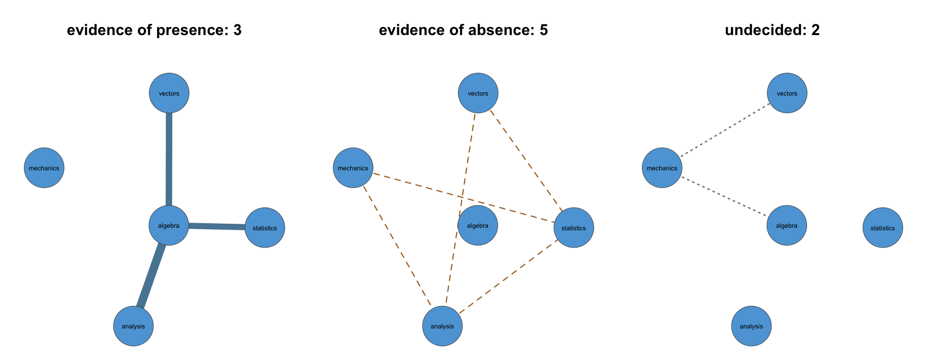
Eighty-eight students is not much data for ten pairs, and the display says so. Three pairs are supported, and all three run through algebra. Five are ruled out: the four pairs that cross between the mechanics-vectors side and the analysis-statistics side, plus analysis-statistics itself. Two are left undecided, mechanics-algebra and mechanics-vectors, with Bayes factors of about 1.2 and 1.0: the data barely move either pair off its prior.

A non-empty undecided panel is a feature of this display, not a defect of the fit. Those two pairs are exactly where a thresholded drawing would have misled you: mechanics-algebra has a posterior inclusion probability of 0.55 and mechanics-vectors of 0.502, both just above one half, so the median probability model would have drawn both as present edges, indistinguishable from the three pairs the data actually support. Two pairs the data cannot decide would have been drawn as if they were settled.

One convenience specific to continuous data: on this fit the Bayes factor is the posterior inclusion odds. Under the default precision_graph_prior = "hierarchical" the prior over structures is exactly the edge prior, so with bernoulli_prior(0.5) the prior inclusion probability of a continuous edge is 0.5 and the prior odds are one. That does not hold under precision_graph_prior = "joint"; extract_inclusion_bf() divides out the right prior odds in either case. See Edge Selection for what to do if you compute the Bayes factor by hand.

Next steps

References

Epskamp, S., Cramer, A. O. J., Waldorp, L. J., Schmittmann, V. D., & Borsboom, D. (2012). qgraph: Network visualizations of relationships in psychometric data. Journal of Statistical Software, 48(4), 1–18. https://doi.org/10.18637/jss.v048.i04
Mardia, K. V., Kent, J. T., & Bibby, J. M. (1979). Multivariate analysis. Academic Press.