Before interpreting results from bgm() or bgmCompare(), check that the MCMC sampler has converged and that posterior estimates are reliable. This chapter describes how to do so with the diagnostic tools in bgms. For background on MCMC convergence diagnostics and choosing the number of iterations, chains, and warmup length, see Margossian & Gelman (2024).
ESS estimates match coda::effectiveSize(Plummer et al., 2006) and R-hat is the split-R-hat of Vehtari et al. (2021): each chain is cut in half and the halves are compared as if they were separate chains. For how both are computed, see the Technical Manual.
Symptom index
Find your symptom, do the one thing in the middle column, then read the linked section for why it is the right thing to do.
Symptom
First thing to do
Where it is explained
Rhat above 1.01
Run longer: raise warmup first, then iter, and keep at least two chains.
Accept the approximation or refit with precision_graph_prior = "joint"; a larger audit (raise bgms.zratio_gauge_sweeps, refit) first tells you whether the flag is noise.
The effective sample size estimates how many independent draws the MCMC chain is equivalent to. Correlated draws reduce the effective information per sample. A larger ESS means more precise posterior estimates (Margossian & Gelman, 2024).
The summary() output reports n_eff for each parameter. How large n_eff needs to be depends on the inferential goal. As a rule of thumb, an ESS of 100 yields an MCSE of roughly \(0.1\) times the posterior standard deviation — enough for one significant digit of precision. An ESS below 100 is also the threshold at which convergence diagnostics such as \(\hat{R}\) and the ESS estimate itself become unreliable (Margossian & Gelman, 2024; Vehtari et al., 2021). If higher precision is required, more iterations or chains are needed: two significant digits require an ESS on the order of 10,000 (Margossian & Gelman, 2024).
Composite ESS for edge-selected parameters
When edge selection is active, pairwise effects are governed by spike-and-slab priors. The parameter is set to exactly zero when the edge is excluded, creating a chain that mixes between zero and nonzero values.
For such a parameter the pairwise table reports a single n_eff, and it is built differently than for an ordinary chain. To the standard autocorrelation machinery, the switching between zero and nonzero values looks like fast mixing, so the ESS comes out too large exactly where the indicator rather than the weight drives the variability. The package instead combines the two sources of Monte Carlo error that limit the model-averaged weight — how well the chain resolved whether the edge is in, and how well it resolved the weight given inclusion — into one equivalent sample size. The companion column share_incl tells you which source dominates. mean, sd, and Rhat are computed from the full chain, zeros included. See Model Output for the columns.
The retired mixture ESS. Earlier versions reported a second, transition-based statistic beside n_eff. It modeled the on/off indicator sequence as a simple two-state process and scored the chain’s switch rates against an independent chain with the same inclusion probability (van den Bergh et al., 2026). That simple process turns out to describe many edge chains poorly, so the statistic could mislead, and 0.2.0.0 retires it: the n_eff_mixt column is gone from the summary tables, and extract_ess(fit, estimator = "mixt") is deprecated. The precision of the inclusion probability and of its Bayes factor is carried by the Rao-Blackwellized n_eff and mcse; the exploration it used to measure is read from the directional transition counts n0->1 and n1->0, which stay in summary(fit)$indicator.
How often an indicator flips mainly reflects the inclusion probability itself: flips are most frequent near 0.5, and an edge with an inclusion probability near 0 or 1 flips rarely even under perfect mixing. A low flip count is therefore not on its own a sign of trouble. Do note the asymmetry between the two directions, which no single summary number can show.
At the extreme, the indicator never switches at all. Even that is not necessarily a problem: when the posterior strongly favors inclusion or exclusion, there is little uncertainty about the indicator, and the inclusion probability is well determined without any switching. For these zero-flip edges the verdict rests on the inclusion probability itself and on extract_inclusion_bf(), which stays finite where the probability saturates.
Inclusion ESS and the exploration counts
For edge indicators the summary table reports its precision columns (mcse, n_eff, Rhat) on the Rao-Blackwellized inclusion draws rather than on the binary indicators. Those draws are continuous, so the standard continuous machinery applies to inclusion inference (see Model Output).
Precision and exploration are still two different questions, and the table answers them in two different places:
n_eff measures precision conditional on exploration. A chain stuck in one region of model space can still produce a smooth, well-converged Rao-Blackwellized chain with a large n_eff.
n0->1 and n1->0 measure the exploration itself.
A confident n_eff beside near-zero transition counts is the boundary signature: a precise one-step estimate resting on little transition evidence. On a saturated edge that is the expected reading rather than a fault.
The Rao-Blackwellized columns come back NA when the inclusion draw barely varies: the chain is certain about the edge, and there is no remaining precision to estimate. Depending on how completely the draw is pinned, either all of mcse, n_eff, and Rhat are NA, or Rhat survives while mcse and n_eff do not. The reading is the same either way: the inclusion probability is pinned, not poorly estimated. These are not the same edges as the zero-transition ones — an indicator that never flipped can still leave a draw with enough variability to summarize.
extract_ess() returns the Rao-Blackwellized n_eff for indicators, so its indicator element lines up with the summary table’s n_eff column and with extract_rhat(), which reads the same continuous chain.
When transitions are observed but rare, the ESS estimate itself becomes imprecise: small fluctuations in the transition counts can produce large swings in the ESS. In these cases, plotting the cumulative inclusion probability across iterations provides a more informative check on stability: a flat trajectory indicates the estimate has settled, while a drifting one suggests the chain needs more iterations.
Monte Carlo standard error (MCSE)
The MCSE measures the additional variability introduced by using a finite number of MCMC draws instead of the exact posterior. It depends on both the posterior variability and the effective sample size.
The same formula covers inclusion probabilities: because the reported estimate is the average of the continuous Rao-Blackwellized inclusion draws rather than of the binary indicators, its sd and n_eff are those of that continuous chain (see Inclusion ESS and the exploration counts). Edges whose inclusion probability is pinned at its bound report NA here.
A small MCSE relative to the posterior standard deviation indicates stable estimates; a large MCSE suggests that more iterations are needed.
R-hat
R-hat compares the between-chain and within-chain variance (Gelman & Rubin, 1992). Values close to 1.0 indicate that the chains have converged to the same distribution; values above 1.01 suggest that the chains have not mixed and should be run longer (Vehtari et al., 2021).
bgms computes the split version of R-hat (Vehtari et al., 2021): each chain is cut in half and the halves enter the comparison as separate chains. This makes the diagnostic sensitive to within-chain drift — a single chain that slowly trends will disagree with its own second half, even if all chains happen to end up in the same place.
The statistic is the classic form. With \(W\) the mean within-sub-chain variance, \(B\) the between-sub-chain variance, and \(n\) draws per sub-chain,
R-hat is reported in summary() output and through extract_rhat(). It is NA when only one chain was run, and when a parameter is constant at the same value in every chain — for example, a pairwise effect whose edge was never included in any chain, so every draw is zero. Constant chains carry no mixing information, so no value is reported rather than a misleading one. If chains are instead stuck at different constant values, R-hat is +Inf: that is a real mixing failure, and it is reported loudly rather than hidden.
For edge indicators, the reported R-hat is computed on the continuous Rao-Blackwellized inclusion draws, and is NA where those draws are exactly constant (see above).
Trace plots
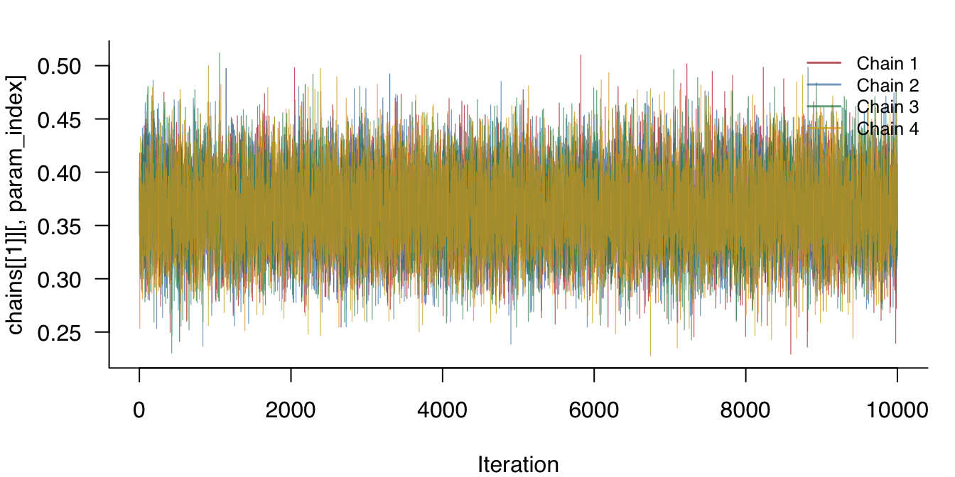
Visually inspecting the sampled values across iterations is a direct way to assess convergence. Chains that have converged look like random noise fluctuating around a stable mean; chains that have not converged show trends, level shifts, or poor mixing.
Raw samples are accessible through fit$raw_samples. The examples on this page use a model fitted to the Wenchuan dataset (17 PTSD symptom items; of the 362 respondents, the 344 with complete data enter the fit under the default na_action = "listwise"):
library(bgms)fit =bgm(Wenchuan, iter =1e4, warmup =5e3, seed =123)
Figure 1: Trace plot for the first pairwise interaction parameter across four chains.
NUTS-specific diagnostics
When using update_method = "nuts" (the default), additional diagnostics are stored in fit$nuts_diag.
E-BFMI
E-BFMI (Energy Bayesian Fraction of Missing Information) measures how efficiently the sampler explores the posterior (Betancourt, 2016). It compares the typical size of energy changes between successive samples to the overall spread of energies. Values close to 1 indicate efficient exploration; values below 0.3 suggest the sampler may be getting stuck (Betancourt, 2017).
A low E-BFMI does not necessarily mean the results are wrong, but it does warrant investigation. In models with edge selection, the most common cause is that the warmup period was too short for the discrete graph structure to equilibrate. Increasing warmup often resolves this.
Divergent transitions
Divergent transitions occur when the numerical integrator encounters regions where the posterior curvature changes too rapidly for the current step size. A small number of divergences (fewer than 0.1% of samples) is generally acceptable. Many divergences indicate that the sampler may be missing important parts of the posterior.
If divergences are frequent, increase target_accept (which reduces the step size). If that does not help, try update_method = "adaptive-metropolis" and compare results.
Mean acceptance probability
fit$nuts_diag$accept_prob is a chains × iterations matrix of the mean acceptance probability across every leapfrog step in each trajectory. The per-chain mean is also reported in fit$nuts_diag$summary. After warmup the per-chain mean should be close to target_accept (default 0.80); a chain whose mean acceptance is materially below the target is a signal that the automatic step-size tuning did not converge — usually because warmup was too short or the geometry has features that warrant a higher target.
Tree depth
NUTS builds trajectories by repeatedly doubling their length until a U-turn criterion is satisfied. If the trajectory frequently reaches the maximum allowed depth (nuts_max_depth), the sampler may benefit from longer trajectories. Hitting the maximum depth occasionally is normal; hitting it on most iterations may indicate challenging posterior geometry. Consider increasing nuts_max_depth.
Warmup equilibration check
In models with edge selection, the discrete graph structure may take longer to reach stationarity than the continuous parameters. Even after warmup completes, the first portion of the sampling phase may still show transient behavior.
The fit$nuts_diag$warmup_check component provides diagnostics comparing the first and second halves of the post-warmup samples:
Field
Meaning
warmup_incomplete
TRUE if any indicator below suggests non-stationarity
energy_slope
Slope of energy vs. iteration; near zero = stable
slope_significant
TRUE if energy slope is significant (p < 0.01)
ebfmi_first_half
E-BFMI for the first half of post-warmup samples
ebfmi_second_half
E-BFMI for the second half
var_ratio
Ratio of energy variance (first half / second half); > 2 suggests settling
Each field is a vector with one entry per chain. With very short runs — fewer than 20 usable post-warmup iterations in a chain — there is too little energy history to split and assess, so the diagnostics for that chain are NA and no flag is raised. An NA here means “not enough draws to check”, not “no problem found”.
If these diagnostics suggest the chain was still settling, increase warmup and refit. If diagnostics remain problematic after doubling or tripling warmup, try refitting with update_method = "adaptive-metropolis" and compare posterior summaries. If the two samplers produce similar results, the estimates are likely trustworthy despite the warnings; if they differ, further investigation is warranted.
The flag on this page’s own fit
The Wenchuan fit used throughout this page raises the flag, which makes it a useful worked case rather than an embarrassment. Here is what it says:
One chain has an energy slope that is statistically significant, so the fit is flagged. Nothing else in the check is out of range: the variance ratios sit near 1, well below the 2 that indicates a chain still settling, and the E-BFMI values are far above 0.3. The message the sampler prints tells you where to look next, and that check is the one that decides. For indicators, extract_ess() and extract_rhat() both read the Rao-Blackwellized inclusion chain, so the indicator row below is two summaries of the same draws:
Every R-hat is below 1.01 and the smallest effective sample size is around a thousand, so the chains agree with each other and with their own halves. The transition counts back that agreement up: of the 136 edges, the 120 the data did not decide outright all moved between structures in both directions, though the slowest of them managed only one flip each way.
A significant energy slope in one chain out of four, with clean R-hat and ESS, is a sensitive detector firing on a real but small trend, not a reason to distrust the posterior. The flag is a prompt to run the two checks above, not a verdict on its own. If R-hat or ESS had also been poor, the remedy would be the one in the previous paragraph: more warmup, then a different sampler.
Trust gauge for the hierarchical graph prior
This check applies to continuous (GGM) and mixed models fitted with edge selection under the default precision_graph_prior = "hierarchical". Under that prior, every edge move evaluates a normalizing-constant ratio through a fast approximation built at the start of the analysis (see the Technical Manual). The trust gauge audits that approximation: two assessment sweeps redo a capped subset of each chain’s own edge decisions with the exact calculation and check whether the approximation changed any of them.
The gauge runs by default, so a default continuous or mixed fit already carries its result:
fit =bgm(data, variable_type ="continuous", ...)fit$zratio_diag
It is silent when clean and prints only flagged chains. Its cost is fixed per chain rather than proportional to iter — nothing on a sparse posterior, and seconds per chain on a dense one at 100 to 200 variables. That is negligible against a production-length fit and noticeable on a short exploratory one, which is what the off switch is for:
options(bgms.zratio_gauge_sweeps =0L)
The summary reports two channels per chain:
flip_rate — the fraction of audited add/remove decisions that would have come out differently under the exact calculation. A chain above 1% is flagged.
harm_pred — the projected distortion of the mean posterior inclusion probability, in probability units, flagged above 0.02. This channel catches a consistent error that shifts the recovered network without changing individual edge decisions, which flip_rate cannot see.
Small values on both channels mean the approximation did not meaningfully affect the sampled graphs. A flagged chain prints the measured error and what the audit covered, followed by advice in order: first raise options(bgms.zratio_gauge_sweeps) and refit, to see whether the signal is real; only after that consider precision_graph_prior = "joint", which is a different model rather than a fix. The gauge never switches specification on its own. See summarize_zratio_gauge() for the full output format and thresholds.
What the sampler’s warnings mean
The lists below cover the warnings a fit and its checks can raise in 0.2.0.0. They are ordinary R warnings, so they surface after the call returns, unlike the NUTS issues: block and the trust gauge report, which the sampler prints while it runs and which the sections above explain. The simulation and prediction helpers carry their own warnings, which are not part of this list.
Warmup is too short for part of the adaptation
These five fire before sampling starts, under update_method = "nuts" with verbose = TRUE (the default; verbose reads getOption("bgms.verbose", TRUE)). Each names the part of warmup adaptation that your warmup is too short to run. The action is the same for all five: raise warmup, using the threshold the message quotes as the floor and the suggestion as the target.
Warning
When it fires
warmup = <n> is very short for edge selection. Consider >= 300.
warmup = <n>: no mass matrix estimation (needs >= 20).
Edge selection off, warmup below 20
warmup = <n>: using proportional allocation (needs >= 150 for fixed buffers).
Edge selection off, warmup from 20 to 149
A chain did not finish
Warning
What to do
<k> of <n> chain(s) failed and will be dropped.
The fit is built from the surviving chains only. R-hat needs at least two, so refit if too few are left for the diagnostics you need. If every chain fails the call stops instead, and the message carries the first chain’s error.
Stopped sampling after user interrupt, results are likely uninterpretable.
Discard the object and refit. The chains stopped wherever the interrupt reached them, so the draws are not a posterior sample.
The normalizing-constant correction could not be built
Continuous and mixed fits that combine edge selection with a Beta-Bernoulli or Stochastic-Block edge prior run their edge-prior updates with a normalizing-constant correction, built at the start of the analysis from a tilted prior sweep; a fit that builds it silently is running corrected. These two warnings mark the cases where the correction cannot be built. The chains still run, but the edge-prior updates lose the correction that keeps them exact, so read the inclusion probabilities as approximate.
Warning
What to do
The <edge prior> updates are run without the normalizing-constant correction: the tilted prior sampler supports only cauchy_prior() and normal_prior() interaction priors.
Refit with interaction_prior = cauchy_prior() or normal_prior() if you want the corrected updates. Reaching this warning at all takes precision_graph_prior = "joint", because the default "hierarchical" rejects any other slab with an error rather than a warning.
The Stochastic-Block updates are run without the normalizing-constant correction: the slope curve is not resolvable for this model cell (a single tilted pair).
Nothing in the call to change: the correction table could not resolve its slope curve for this combination of size and prior. Read the block structure as approximate, and compare it against a Beta-Bernoulli fit of the same data before reporting it.
The z-ratio tables left their certified range
Both fire while the hierarchical graph prior builds its approximation, on a fit whose precision diagonal shape is not 1. They say the approximation behind every edge move may be less accurate than certified, so check fit$zratio_diag before reading the graph; see the trust gauge.
Warning
What to do
Z-ratio constants at diagonal shape <a> lie outside the certified range [0.5, 20]; the fixed quadrature grids are not scored there and may lose accuracy.
Bring the diagonal shape back inside 0.5 to 20 if the analysis allows it. Otherwise treat the gauge as the check that decides.
Z-ratio pair integrals retain visible mass at the grid edge (delta = <d>, eta = <e>, shape = <a>); the saddle tables may be truncated.
Same reading: the quadrature grid did not capture the whole integrand at this prior setting, so let the gauge decide whether it mattered.
The data cannot support part of the model
Warning
What to do
Blume-Capel variable <name> has <k> categories. This may slow computation. Empty categories are not collapsed.
Nothing is wrong with the fit; expect it to be slower. Fires above 10 categories. Empty categories in the range still cost time, so collapse them yourself if they are an artifact of coding.
Some categories were not used by every group: ...
A bgmCompare() warning. The threshold differences it names rest on the prior rather than on the data. Do not read them as evidence of a group difference; the printed summary marks the rows with *, and extract_arguments(fit)$category_support holds the per-group counts. Pairwise differences are unaffected. It carries the condition class bgms_group_support_warning, so you can catch this one warning without muffling the rest.
A deprecated argument
The arguments the 0.2.0 prior objects replaced still work, and warn through lifecycle naming their replacement:
The `pairwise_scale` argument of `bgm()` is deprecated as of bgms 0.2.0.
Please use the `interaction_prior` argument instead.
Nothing about the fit is wrong. Move the call to the replacement so it keeps working past the deprecation; the full mapping is on bgm() and bgmCompare().
The checks and the ecosystem
Warning
What to do
The usable radii of the <a>x and <b>x anchors do not overlap; the curve has a gap between them. Add an anchor in that range.
From prior_sensitivity_check(). Rerun with an extra anchor between the two the message names, so the curve is continuous there.
easybgm <version> is not compatible with S7-based bgms objects. Running in S3 compatibility mode. Please update easybgm to version 0.5.0 or later.
Update easybgm. Until then the fit is returned as a plain list, so the S7 accessors this documentation uses will not all apply.
Results differ between runs
Two runs of the same call differ for one of two reasons, and the remedy differs with them.
If you did not set seed, the runs drew different random numbers and small differences are expected. Pass a single non-negative integer to seed to make a run repeatable.
If you did set seed and the runs still differ, the guarantee is narrower than it looks, and bgm() states its exact scope. Results are bit-reproducible for a given installed binary; they are not portable across compilers or optimization settings, so a rebuilt or reinstalled binary can produce different draws from the same seed, with the differences concentrated where the posterior is weakly identified. On Windows with RcppParallel 6.0.0 or later, a fixed seed reproduces a run only at the same cores setting: runs at different core counts are statistically equivalent, not identical.
Differences that survive all of that, and that change what you would report, are a mixing problem rather than a seeding one. Two runs landing on different answers is what R-hat is built to detect across chains, so check R-hat and ESS first and treat the run-to-run gap as the same failure seen from outside.
Run-length settings
Three bgm() arguments control how much sampling is done:
Argument
Default
What it controls
warmup
2000
Adaptation iterations per chain (discarded)
iter
2000
Post-warmup draws kept per chain
chains
4
Independent chains run in parallel
When diagnostics indicate a problem, match the remedy to the symptom:
Low ESS or an MCSE that is large relative to the effects you care about — increase iter; precision grows with the number of retained draws.
Warmup warnings in fit$nuts_diag$warmup_check, persistent divergences, or acceptance below target — increase warmup; the sampler needs more adaptation time, and extra post-warmup draws will not fix a poorly tuned sampler.
R-hat above 1.01 — first check the trace plots; if chains disagree, longer warmup (and sometimes longer iter) is the remedy. Keep at least two chains — with a single chain, R-hat cannot be computed.
Recommended workflow
Inspect summary(): check R-hat (< 1.01) and ESS (≥ 100) for all parameters.
Check NUTS diagnostics: fit$nuts_diag$summary for divergences, tree depth saturation, E-BFMI, and a mean acceptance probability (mean_accept_prob) close to target_accept. The fit$nuts_diag$has_issues flag is TRUE when any of these checks raised a concern.
Check warmup: fit$nuts_diag$summary$warmup_incomplete and the per-chain detail in fit$nuts_diag$warmup_check for signs of incomplete equilibration.
Plot traces: visually inspect a few key parameters for mixing and stationarity.
On a continuous or mixed fit: check fit$zratio_diag for flagged chains. The trust gauge fills it by default.
If problems are found: increase warmup and/or iter, adjust target_accept, or switch samplers.
Still stuck
If longer warmup and more iterations have not moved the diagnostics, refit with the other sampler and compare:
How to read the comparison is in the warmup equilibration check: if the two samplers produce similar posterior summaries, the estimates are likely trustworthy despite the warnings, and if they differ, the disagreement is itself the finding and nothing should be reported until it is resolved.
If that leaves you stuck, ask on the bgms issue tracker. A report that can be acted on carries the bgm() call as you ran it, fit$nuts_diag$summary, and the output of sessionInfo().
References
Betancourt, M. (2016). Diagnosing suboptimal cotangent disintegrations in Hamiltonian Monte Carlo. arXiv Preprint. https://arxiv.org/abs/1604.00695
Gelman, A., & Rubin, D. B. (1992). Inference from iterative simulation using multiple sequences. Statistical Science, 7(4), 457–472. https://doi.org/10.1214/ss/1177011136
van den Bergh, D., Clyde, M. A., Raftery, A. E., & Marsman, M. (2026). Reversible jump MCMC with no regrets: Bayesian variable selection using mixtures of mutually singular distributions. Manuscript in Preparation.
Vehtari, A., Gelman, A., Simpson, D., Carpenter, B., & Bürkner, P.-C. (2021). Rank-normalization, folding, and localization: An improved \(\widehat{R}\) for assessing convergence of MCMC (with discussion). Bayesian Analysis, 16(2), 667–718. https://doi.org/10.1214/20-BA1221