Methods

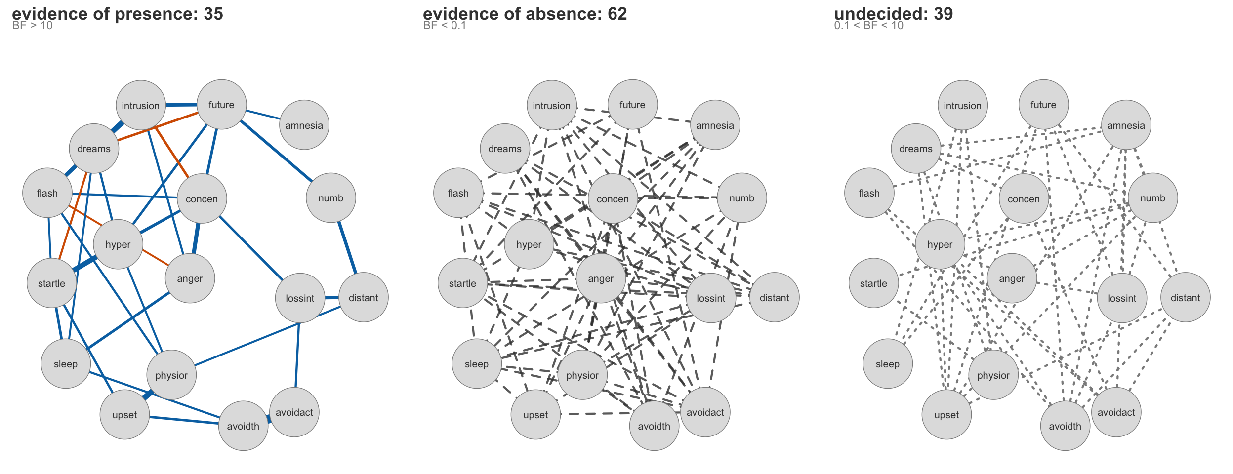
Methods for inspecting, summarizing, and using bgms and bgmCompare model fits. Both are S7 classes; methods use S3 dispatch for compatibility with base R generics.

print

print(x, ...)

Argument	Description
x	An object of class bgms or bgmCompare.
...	Ignored.

Returns x invisibly.

summary

summary(object, ...)

Argument	Description
object	An object of class bgms or bgmCompare.
...	Currently ignored.

Returns a summary object containing:

• main — Data frame of main-effect summaries: mean, mcse, sd, n_eff, Rhat.
• pairwise — Data frame of partial association summaries. With edge selection the parameter is the model-averaged edge weight, so mcse and n_eff are composite quantities and the table adds share_incl, the share of the squared Monte Carlo error owed to inclusion rather than slab uncertainty.
• indicator — Data frame of inclusion indicator summaries (if edge/difference selection enabled): mean, mcse, sd, n_eff, Rhat, n0->1, n1->0. The mean, mcse, sd, and n_eff columns are computed on the Rao-Blackwellized inclusion draws; n0->1 and n1->0 count transitions of the binary indicator chain and carry the exploration signal. The precision columns come back NA where the inclusion probability is pinned and no precision is left to estimate: mcse, n_eff, and Rhat when the draws are exactly constant, and mcse and n_eff alone when the draws vary too little for the autocorrelation machinery. The transition-based n_eff_mixt column was dropped in 0.2.0.0.

See Model Output for how to read these columns.

For bgmCompare, summaries are split into baseline and difference components: main and pairwise carry the baseline parameters, while main_diff and pairwise_diff carry the differences and, being the selected parameters there, are the tables that report share_incl.

coef

Extract posterior mean coefficients.

coef(object, ...)

Argument	Description
object	An object of class bgms or bgmCompare.
...	Ignored.

Returns (by class):

• bgms: main, pairwise, and (if available) indicator.
• bgmCompare: main_effects_raw, pairwise_effects_raw, main_effects_groups, pairwise_effects_groups, and indicators.

plot

Draw the fitted model. The default display is the network split by what the data settle about each pair.

plot(x, type = c("network", "centrality"), evidence_threshold = 10,
     layout = "spring", ...)

plot(x, type = c("difference", "groups", "centrality"),
     evidence_threshold = 10, group = 1, layout = "spring",
     max_panels = 3L, page = 1L, ...)

Argument	Description
x	An object of class bgms or bgmCompare.
type	Which display to draw. bgms: "network" (default) or "centrality". bgmCompare: "difference" (default), "groups", or "centrality".
evidence_threshold	Numeric greater than 1. The inclusion Bayes factor separating evidence of presence from undecided, as in verdicts(). Default: 10.
group	bgmCompare only, for type = "centrality": a single group index passed to extract_centrality(). Default: 1.
layout	Layout passed to qgraph::qgraph(). Default: "spring".
max_panels, page	bgmCompare only, for type = "groups": how many group networks are drawn at once, and which page of them. Defaults 3 and 1.
...	Passed to qgraph::qgraph(), or to plot() on the centrality object for type = "centrality".

Returns x invisibly; called for the side effect of drawing. Drawing the network needs the suggested package qgraph.

The edge evidence plot

type = "network" is the edge evidence plot: three panels on one shared layout holding the pairs the data support, the pairs the data rule out, and the pairs the data cannot decide. It is the canonical result display this documentation uses for every network, and plot() is its in-package implementation: the classification is the one verdicts() reports at the same evidence_threshold, each panel is titled with what it holds and how many pairs are in it, and the layout is computed once from every pair so a node sits in the same place in all three panels.

Only the first panel is weighted. There, line width is the posterior mean pairwise association and color carries its sign, blue for positive and vermillion for negative, the Okabe-Ito pair, so the sign survives common forms of color-vision deficiency. The other two panels are drawn at uniform width, dashed for evidence of absence and dotted for undecided: for those pairs the classification is the result, and a width would suggest an effect size the data have either ruled out or not established.

The figure carries no key: each panel’s title names the evidence class and its count, with the classification rule printed beneath it.

For the same display built by hand with qgraph, and for the reasoning behind it, see the plot_edge_evidence() helper in Getting Started and Edge Selection.

Device size. Three networks side by side need a wide device. R’s default 7 by 7 inches leaves each panel a little over two inches, and at that size the labels and titles crowd; plot() says so when the device is too small. Open a wider device before plotting:

dev.new(width = 13, height = 5)   # or pdf(f, width = 13, height = 5)
plot(fit)

Without edge selection there is no indicator and nothing to split the pairs by, so plot() draws one panel with every pair on it, width the posterior mean association and color its sign, titled "Edge weights".

Example

plot(fit)

Figure 1: The edge evidence plot for the Wenchuan fit: 35 pairs supported, 62 ruled out, 39 undecided at an inclusion Bayes factor of 10.

plot(fit, type = "centrality")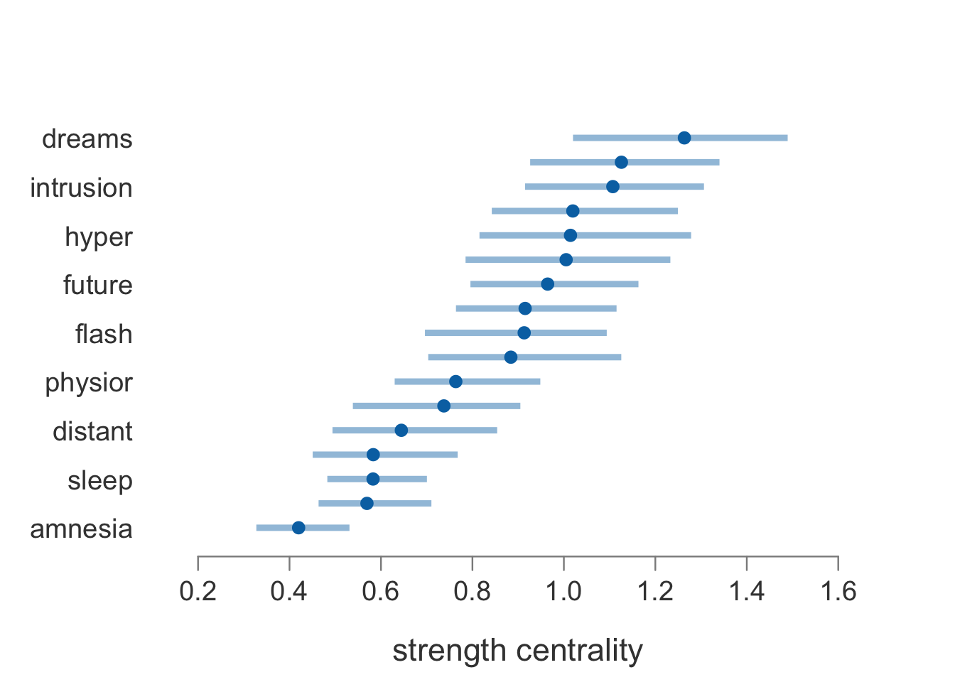

Figure 2: Posterior strength centrality for the same fit.

bgmCompare displays

On a bgmCompare fit the default type = "difference" is the same three-panel display read for differences: the pairs whose difference the data support, rule out, and cannot decide. Which group a positive difference favors follows the contrast coding, which extract_group_params() reports per group.

Two cases change the picture. With more than two groups a pair has \(K - 1\) posterior mean differences rather than one, so no single number is “the” difference and the first panel is drawn unweighted; read the magnitudes per group with type = "groups" or extract_group_params(). When main_difference_selection = TRUE gave main-effect differences their own indicators, their evidence is carried on the nodes: each node wears a ring filled to its difference indicator’s posterior inclusion probability and colored by the verdict. Under the default main_difference_selection = FALSE those indicators do not exist and no ring is drawn.

type = "groups" draws each group’s own posterior mean network on the layout the difference display uses. Those panels are estimates, not evidence, so every pair is drawn with its weight.

plot_edge_posterior

Draw one edge’s weight the way JASP draws a parameter: the posterior density against the prior it was updated from, with the evidence for the edge as a filled probability wheel and the estimate printed beside it.

plot_edge_posterior(bgms_object, variable1, variable2, ...)

Argument	Description
bgms_object	A fitted bgms object from bgm().
variable1, variable2	The two variables naming the edge, as names or column positions.
binwidth	Deprecated. The panel no longer expresses the weight as probability per bin, so this has nothing to set; it is warned about and ignored.
...	Ignored.

Returns bgms_object invisibly; called for the side effect of drawing.

The panel shows two curves on one density scale. The solid accented curve is the posterior of the edge weight; the dashed grey curve is the prior it was updated from, computed in closed form from the fit’s own interaction_prior rather than assumed, so a panel drawn from a cauchy_prior(scale = 2.5) fit and one drawn from the default normal_prior(scale = 1) do not look alike.

What the curves mean follows the model the fit actually used. With edge selection the posterior of the weight is a spike-and-slab, and the panel draws the continuous part conditional on the edge being included, which is a genuine density integrating to one. The mass at zero is carried by the probability wheel, whose accented share is the posterior inclusion probability. The evidence is printed as the natural log of the inclusion Bayes factor from extract_inclusion_bf(), which bgms estimates by Rao-Blackwellizing the indicator draws. It is not a ratio of densities at zero, so the panel does not draw Savage-Dickey ordinates. Without edge selection there is no point mass, the Savage-Dickey density ratio is the licensed estimator, and the panel marks both ordinates at zero with grey dots and prints their ratio on the same natural-log scale.

The median and 95% credible interval printed at the top right are of the same posterior the density shows. An edge the data rule out is still drawn: when no retained draw included it there is no conditional posterior to show, so the panel draws the prior, the wheel and the evidence, and the missing accented curve is itself the statement.

No verdict word is printed. The panel shows the evidence and leaves the reading to the threshold you choose; verdicts() is where the package states verdicts, and it names the threshold it used.

Example

plot_edge_posterior(fit, "intrusion", "dreams")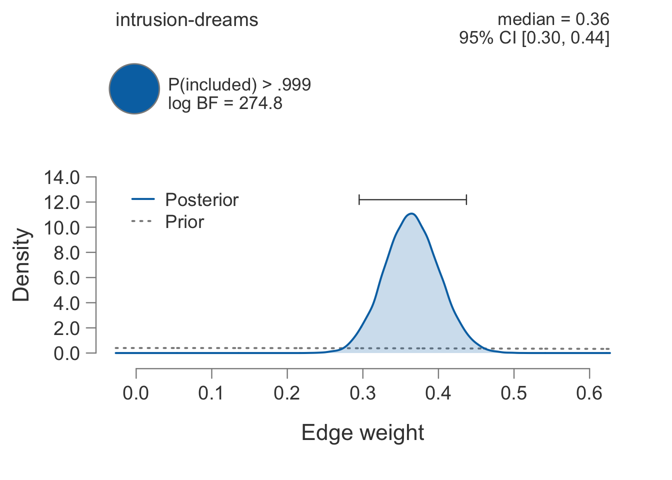

Figure 3: The posterior of the intrusion-dreams edge weight against its prior, with the inclusion evidence as a probability wheel.

predict

Compute conditional probability distributions for one or more variables given the observed values of other variables in the data.

predict(object, newdata, variables = NULL,
        type = c("probabilities", "response"),
        method = c("posterior-mean", "posterior-sample"),
        ndraws = NULL, seed = NULL, ...)

predict(object, newdata, group, variables = NULL,
        type = c("probabilities", "response"),
        method = c("posterior-mean"), ...)

Argument	Description
object	An object of class bgms or bgmCompare.
newdata	A matrix or data frame matching the variables used in fitting.
group	Integer group index for bgmCompare only (required there).
variables	Character names, integer indices, or NULL (all variables).
type	"probabilities" or "response".
method	bgms: "posterior-mean" or "posterior-sample"; bgmCompare: "posterior-mean".
ndraws	For bgms with method = "posterior-sample".
seed	Optional random seed.

Return shape depends on model type:

• Ordinal: probabilities per category or predicted categories.
• GGM: conditional means/sds or conditional means.
• Mixed: combined discrete and continuous outputs.

For bgmCompare, outputs use group-specific parameters (baseline plus group differences).

Example

# Predict probabilities for the first observation's variable 1
# given its observed values on variables 2-17
predict(fit, newdata = Wenchuan[1, , drop = FALSE], variables = 1)

$intrusion
         cat_0     cat_1     cat_2      cat_3        cat_4
[1,] 0.1047114 0.6530421 0.2099615 0.03154664 0.0007383951

# Predict responses (most likely category) for first 3 observations
predict(fit, newdata = Wenchuan[1:3, ], variables = 1:3, type = "response")

     intrusion dreams flash
[1,]         1      1     1
[2,]         1      1     1
[3,]         3      1     2

simulate

Generate new observations from a fitted model.

simulate(object, nsim = 500, seed = NULL,
         method = c("posterior-mean", "posterior-sample"),
         ndraws = NULL, iter = 1000,
         cores = parallel::detectCores(),
         display_progress = c("per-chain", "total", "none"), ...)

simulate(object, nsim = 500, seed = NULL, group,
         method = c("posterior-mean"), iter = 1000, ...)

Argument	Description
object	An object of class bgms or bgmCompare.
nsim	Number of observations to simulate. Default: 500.
seed	Optional random seed.
group	Integer group index for bgmCompare only (required there).
method	bgms: "posterior-mean" or "posterior-sample"; bgmCompare: "posterior-mean".
ndraws	For bgms with method = "posterior-sample".
iter	Gibbs iterations for equilibration. Default: 1000.
cores, display_progress	Used for bgms with method = "posterior-sample".

Returns:

• bgms, posterior-mean: matrix (nsim x p).
• bgms, posterior-sample: list of matrices (one per draw).
• bgmCompare: matrix (nsim x p) for the selected group.

Discrete columns are returned on the original category scale of the training data (the values supplied to bgm()), not the internal 0, 1, ..., m recoding, so the output can be passed straight to predict(). For mixed MRF models, discrete columns contain non-negative integers and continuous columns contain real-valued observations, ordered as in the original data.

Example

# Fit a model
fit = bgm(Wenchuan, iter = 1e4, warmup = 5e3, seed = 123)

# Simulate 100 new observations from the posterior mean network
sim_data = simulate(fit, nsim = 100, seed = 42)
head(sim_data)

     intrusion dreams flash upset physior avoidth avoidact amnesia lossint
[1,]         3      3     4     3       5       3        3       4       2
[2,]         4      4     3     2       2       3        2       1       2
[3,]         2      2     2     1       1       2        2       1       1
[4,]         2      1     1     1       1       1        2       1       4
[5,]         4      3     2     3       2       4        4       2       2
[6,]         3      1     2     4       4       4        3       2       2
     distant numb future sleep anger concen hyper startle
[1,]       2    1      2     4     3      4     2       4
[2,]       2    2      3     3     2      2     2       2
[3,]       1    1      1     1     3      1     1       1
[4,]       2    1      2     2     2      2     2       2
[5,]       2    2      1     2     3      2     2       2
[6,]       2    2      3     4     5      2     1       3

simulate_mrf

Simulate observations from a Markov Random Field using user-specified parameters (no fitted model needed).

simulate_mrf(
  num_states,
  num_variables,
  num_categories,
  pairwise,
  main,
  variable_type = "ordinal",
  baseline_category,
  iter = 1000,
  seed = NULL
)

Argument	Description
num_states	Number of observations to generate.
num_variables	Number of variables in the MRF.
num_categories	Integer or integer vector. Number of response categories on top of the base category (1 = binary).
pairwise	Symmetric matrix of partial associations. For continuous variables, this is the precision matrix (must be positive definite).
main	Main-effect parameters. For ordinal variables: a matrix of category thresholds. For continuous variables: a means vector.
variable_type	"ordinal", "blume-capel", or "continuous". Can be a vector for mixed types (ordinal/Blume-Capel only).
baseline_category	Integer vector of baseline categories for Blume–Capel variables.
iter	Gibbs iterations for equilibration (ordinal only). Default: 1000.
seed	Optional random seed.

Returns a (num_states x num_variables) matrix of simulated observations.

For ordinal and Blume-Capel variables, the Gibbs sampler generates observations from full conditional distributions. For continuous variables, observations are drawn directly from \(N(\mu, \Omega^{-1})\).

Example

# Simulate from a 3-variable binary MRF with specified parameters
pairwise = matrix(c(
   0.0,  0.5, -0.3,
   0.5,  0.0,  0.4,
  -0.3,  0.4,  0.0
), nrow = 3, byrow = TRUE)

main = matrix(c(0.0, -0.5, 0.2), nrow = 3, ncol = 1)

sim_data = simulate_mrf(
 num_states = 500,
 num_variables = 3,
 num_categories = c(1, 1, 1),
 pairwise = pairwise,
 main = main,
 seed = 123
)
head(sim_data)

     [,1] [,2] [,3]
[1,]    1    1    0
[2,]    1    1    1
[3,]    1    1    1
[4,]    1    1    1
[5,]    0    1    1
[6,]    1    0    0

Deprecated

• mrfSampler() — Renamed to simulate_mrf() in 0.1.6.3. It still works, with the same arguments and return value, and warns once per session.

See also

bgm(), bgmCompare(), extractor functions