Comparing groups

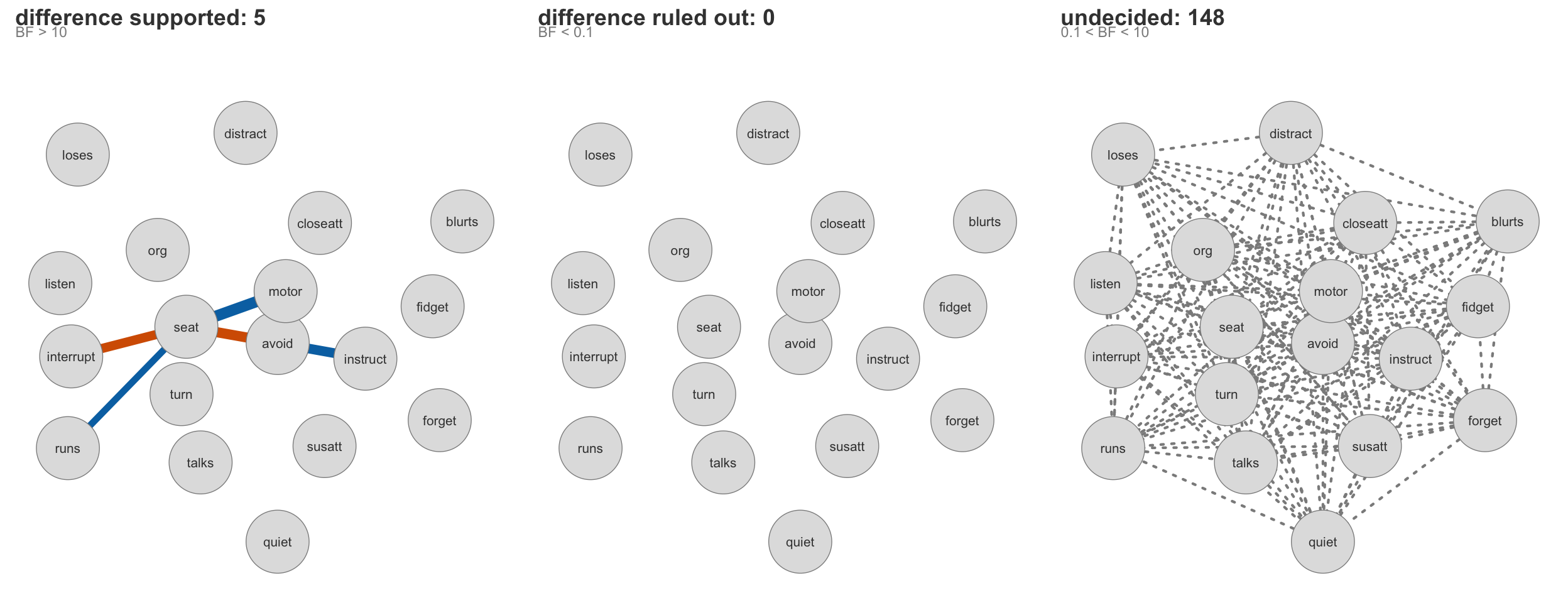
Of the 153 pairwise associations in the ADHD symptom network, the data support a group difference for five, rule none out, and leave 148 undecided. That headline is the page: a comparison that reports, per parameter, whether the groups differ, whether they are credibly the same, or whether these data cannot tell.

“Is the network different between groups?” is really two claims that a comparison should keep apart: this association differs between the groups, and this association is credibly the same. The second claim is the one a significance test cannot make: where the Network Comparison Test asks whether two networks differ somewhere, the Bayesian comparison answers parameter by parameter, and evidence of equivalence becomes expressible. Each pairwise difference gets its own indicator and its own inclusion Bayes factor, read exactly like the edge verdicts of From estimation to evidence, with “difference” in place of “edge”.

The fit

library(bgms)

fit = bgmCompare(
  x = ADHD[, -1],
  group_indicator = ADHD$group,
  variable_type = "ordinal",
  seed = 123
)

The ADHD data ship with the package: 18 binary DISC-IV symptom items for 355 children, 146 with an ADHD diagnosis and 209 without, with group coding the diagnosis. The call is bgmCompare() at its defaults plus a seed, so every number below is what the defaults give you on these data. The run takes a few minutes. The defaults are exploration-length (2,000 warmup, 2,000 sampling iterations); for a published claim, the run-length reasoning of Reading the output applies to difference indicators exactly as it does to edges.

plot(fit)

Read the verdicts

verdicts(fit)

Edge verdicts at an inclusion Bayes factor of 10 (and 0.1 for absence):
presence: log BF > 2.30; absence: log BF < -2.30

  presence 5 | undecided 148 | absence 0   (153 indicators)
  Main-effect differences are not under selection (main_difference_selection = FALSE).

                 parameter   pip log_bf   verdict fragile
 avoid-closeatt (pairwise) 0.861  1.826 undecided   FALSE
 avoid-distract (pairwise) 0.353 -0.606 undecided   FALSE
   avoid-forget (pairwise) 0.809  1.442 undecided   FALSE
 avoid-instruct (pairwise) 0.970  3.480  presence   FALSE
   avoid-listen (pairwise) 0.823  1.540 undecided   FALSE
    avoid-loses (pairwise) 0.480 -0.082 undecided   FALSE
      avoid-org (pairwise) 0.754  1.121 undecided   FALSE
   avoid-susatt (pairwise) 0.680  0.752 undecided   FALSE
   avoid-blurts (pairwise) 0.377 -0.502 undecided   FALSE
   avoid-fidget (pairwise) 0.872  1.918 undecided   FALSE
... (143 more rows)

2 verdicts are Monte-Carlo fragile: a verdict boundary lies within two standard
errors of the evidence, so the verdict could change on a rerun. Consider a
longer run.

The fragility flag is not validated for difference indicators: its
operating point was established on single-network edge indicators only.
Read it as an indication that a verdict sits near a boundary, not as a
calibrated error rate.

Difference verdicts are scale-contingent: group differences are priced
on the association scale through difference_scale, and the calibration
of that default is under study, so a verdict close to a decision
threshold can move with the scale.

The counts are the headline: 5 differences supported, 148 undecided, 0 with evidence of equivalence at the default threshold of 10. The 18 main-effect difference rows print as unsampled: under the default main_difference_selection = FALSE the threshold differences are free parameters, not selected ones, so they carry no indicator to read (the print marks those rows and leaves them out of its counts). Two verdicts are flagged fragile, and the print also notes that the fragility flag’s operating point was calibrated on single-network edge verdicts, not on difference verdicts; the flag still marks verdicts near a boundary, but its error-catching rate is unmeasured here. See verdicts() for both contracts.

The summary(fit) layout follows the single-network fit block by block, and Reading the output owns that walkthrough; what is new here is that the selected parameters are the differences, so the pairwise_diff table is where share_incl and the indicator diagnostics live.

The two directions

A difference, walked. The strongest one is motor-seat, the association between being “on the go, driven by a motor” and leaving one’s seat:

bf = extract_inclusion_bf(fit)
bf["motor", "seat"]

[1] 886.4053

coef(fit)$pairwise_effects_groups["motor-seat", ]

    group1     group2 
-0.5076113  0.9122395

A difference Bayes factor of about 886, and the group-specific model-averaged weights say what the difference is: in the group without a diagnosis the association is negative (about \(-0.51\)), in the diagnosed group strongly positive (about \(0.91\)). The two symptoms travel together among diagnosed children and apart among the others, conditional on the remaining sixteen symptoms. That sign flip, not just its size, is the finding.

Equivalence, honestly. On these data at this run length, no difference reaches evidence of equivalence at the threshold of 10: the strongest lean toward invariance is forget-org at \(\text{BF}_{01} \approx 3.6\), which is still undecided. The claim becomes available at a laxer convention:

table(verdicts(fit, evidence_threshold = 3)$verdict)


 presence undecided   absence 
       25       120         8

At a threshold of 3, eight associations carry evidence of equivalence. State the threshold, and read the claim with the same care as the absence panel of the single-network analysis: it is evidence that the modeled partial association is invariant across the groups, under this model and these priors. It is not a statement that the groups are identical, and an undecided difference is not equivalence; with 148 of 153 differences undecided, the loudest thing these data say is that 355 children decide very little about group differences at this evidence bar.

The three panels

The figure at the top of the page is plot(fit): the same three-panel evidence display as for a single network, read for differences. The first panel holds the five supported differences, weighted by the posterior mean difference; the second holds the differences the data rule out, drawn dashed, and is empty here; the third holds the 148 dotted undecided pairs. A blank in a side-by-side drawing of two estimated networks cannot distinguish “no difference” from “cannot tell”; this display keeps them apart, and on these data the honest panel is the crowded third one.

What to report

For a supported difference: “The partial association between <X> and <Y> differed between the groups (\(\text{BF}_{10} = \texttt{<value>}\)); it was <w1> in <group 1> and <w2> in <group 2>.”
For an equivalence claim: “The data supported invariance of the <X>-<Y> association across groups (\(\text{BF}_{01} = \texttt{<value>}\)),” stating the threshold it clears and the run it rests on.
The counts: how many differences were supported, ruled out, and undecided at your threshold, out of how many possible.
Not licensed: reading an undecided difference as evidence the groups are the same, or a side-by-side pair of estimated networks as a difference test.

Where to next

Group Comparison for the model: the contrast parameterization, difference selection, and the prior on the differences.
bgmCompare() for the arguments and return value, and Reading the output for the shared summary blocks.
A companion tutorial developing the Bayesian group comparison in full is in preparation.
Back in the series: From estimation to evidence, the single-network analysis this page extends.